3.3 Computing the Hazard Ratio
One of the main goals of the Cox PH model is to compare the hazard rates of individuals who have different values for the covariates. The idea is that we care more about comparing groups than about estimating absolute survival. To this end, we are going to use the Hazard Ratio (HR).
A hazard ratio is defined as the hazard for one individual divided by the hazard for a different individual. The two individuals being compared can be distinguished by their values for the set of predictors, that is, the \(X\)’s. We can write the hazard ratio as the estimate of
\[ \widehat{HR} = \frac{\hat h_i(t|\textbf X_i)}{h_j(t|\textbf X_j)} = \frac{\hat h_0(t) \exp (\boldsymbol{\hat \beta} \textbf X_i)}{\hat h_0(t) \exp (\boldsymbol{\hat \beta}\textbf X_j)}=exp(\boldsymbol{\hat \beta}(\textbf X_i - \textbf X_j)). \]
Additionally, we can construct a \((1-\alpha)\)% confidence interval for the hazard ratio as \[ \exp( \boldsymbol{\hat \beta}(\textbf X_i - \textbf X_j) \pm z_{1-\alpha/2} \hspace{0.2cm} \widehat{se}(\boldsymbol{\hat \beta}(\textbf X_i - \textbf X_j)), \] where \(\widehat{se}(\boldsymbol{\hat \beta}(\textbf X_i - \textbf X_j))\) is equal to \(\sqrt{ \widehat{Var}(\boldsymbol{\hat \beta}(\textbf X_i - \textbf X_j))}\).
In order to understand what this hazard ratio means, we are going to see same examples.
In the first one we are using a discrete predictor (smoking) and we will see the hazard ratio for smoking versus not smoking adjusted by the age. So, let \(\textbf X_i:(smoking=1, age = 60)\) and \(\textbf X_j:(smoking=0, age = 60)\), the hazard ratio is
\[ HR= \frac{h_i(t|\textbf X_i)}{h_j(t|\textbf X_j)} = \frac{h_0(t) e^{\beta_{smoking} \cdot 1 + \beta_{age} \cdot 60}}{h_0(t) e^{\beta_{age} \cdot 60}} = e^ {\beta_{smoking}} \]
For example, if \(\beta_{smoking}= 0.5\), the hazard ratio for smoking adjusted for age will be \(exp(0.5)= 1.65\). That is, the hazard of death increases 65% for smokers.
In the second example we use a continuous predictor, age of the individuals. Let \(\textbf X_i:(smoking=0, age = 70)\) and \(\textbf X_j:(smoking=0, age = 60)\), the hazard ratio for a ten years increase in age adjusted by smoking is
\[ HR= \frac{h_i(t|\textbf X_i)}{h_j(t|\textbf X_j)} = \frac{h_0(t) e^{\beta_{smoking} \cdot 0 + \beta_{age} \cdot 70}}{h_0(t) e^{\beta_{smoking} \cdot 0+ \beta_{age} \cdot 60}} = e^{\beta_{age}(70-60)} = e^{\beta_{age}\cdot 10 = (e^{\beta_{age}})^{10} } \]
Note that \(e^{\beta_{age}}\) is the hazard ratio for a 1-unit increase in the predictor.
Interpretation of the hazard ratio (like Odds Ratio in Logistic Models)
- HR = 1: no effect
- HR > 1: increase in the hazard
- HR < 1: reduction in the hazard
Moving again on the R code, we can see (by means of the summary function) the hazard ratios for the covariates included in the model
m1 <- coxph(Surv(time, status) ~ LoanOriginalAmount2 + IsBorrowerHomeowner +
              IncomeVerifiable, data = loan_filtered)
summary(m1)
## Call:
## coxph(formula = Surv(time, status) ~ LoanOriginalAmount2 + IsBorrowerHomeowner +
##     IncomeVerifiable, data = loan_filtered)
##
##   n= 4923, number of events= 1363
##
##                             coef exp(coef) se(coef)      z Pr(>|z|)
## LoanOriginalAmount2     -0.12177   0.88535  0.06661 -1.828   0.0675 .
## IsBorrowerHomeownerTrue -0.24815   0.78025  0.06231 -3.982 6.82e-05 ***
## IncomeVerifiableTrue     0.29263   1.33995  0.30286  0.966   0.3339
## ---
## Signif. codes:  0 '***' 0.001 '**' 0.01 '*' 0.05 '.' 0.1 ' ' 1
##
##                         exp(coef) exp(-coef) lower .95 upper .95
## LoanOriginalAmount2        0.8854     1.1295    0.7770    1.0088
## IsBorrowerHomeownerTrue    0.7802     1.2816    0.6905    0.8816
## IncomeVerifiableTrue       1.3399     0.7463    0.7401    2.4260
##
## Concordance= 0.558  (se = 0.008 )
## Rsquare= 0.005   (max possible= 0.988 )
## Likelihood ratio test= 24.46  on 3 df,   p=1.999e-05
## Wald test            = 23.33  on 3 df,   p=3.44e-05
## Score (logrank) test = 23.46  on 3 df,   p=3.238e-05
termplot(m1, terms = "IsBorrowerHomeowner")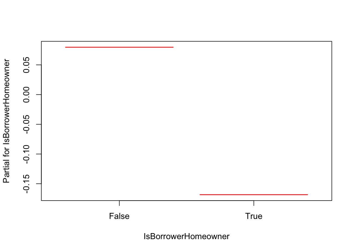
The estimated hazard ratio for IsBorrowerHomeowner == True vs IsBorrowerHomeowner == False is 0.78 with a 95% CI of (0.69, 0.88), that is, IsBorrowerHomeowner == True has 0.78 times the hazard of IsBorrowerHomeowner == False, a 22% lower hazard rate. The estimated hazard ratio for IsBorrowerHomeowner == False vs IsBorrowerHomeowner == True is 1.28. Note that the procedure is the same for the other covariates.