3.7 Non-Proportional Hazards… and now what?
A insignificant nonproportionality may make no difference to the interpretation of a dataset, particularly for large sample sizes. What if the nonproportionality is large and real? Possible approaches are possible in the context of the Cox model itself:
Stratify. Covariates with nonproportional effects may be incorporated into the model as stratification factors rather than predictors (but… be careful, stratification works naturally for categorical variables, however for quantitative variables you would have to discretize).
Partition of the time axis, if the proportional hazards assumption holds for short time periods but not for the entire study.
Nonlinear effect. Continuous covariates with nonlinear effect may lead to nonproportional effects.
3.7.1 An example… Stratified Proportional Hazards Models
Sometimes the proportional hazard assumption is violated for some covariate. In such cases, it is possible to stratify taking this variable into account and use the proportional hazards model in each stratum for the other covariates. We include in the model predictors that satify the proportional hazard assumption and remove from it the predictor that is stratified.
Now, the subjects in the \(z\)-th stratum have an arbitrary baseline hazard function \(h_{0z}(t)\) and the effect of other explanatory variables on the hazard function can be represented by a proportional hazards model in that stratum
\[ h_z(t, \textbf X) = h_{0z}(t) e^{\sum_{j=1}^p \beta_j X_j} \] with \(z = 1, \ldots, k\) levels of the variable that is stratified.
In the Stratified Proportional Hazards Model the regression coefficients are assumed to be the same for each stratum although the baseline hazard functions may be different and completely unrelated.
m3 <- coxph(Surv(time, status) ~ LoanOriginalAmount2 +
strata(IsBorrowerHomeowner), data = loan_filtered)
summary(m3)
## Call:
## coxph(formula = Surv(time, status) ~ LoanOriginalAmount2 + strata(IsBorrowerHomeowner),
## data = loan_filtered)
##
## n= 4923, number of events= 1363
##
## coef exp(coef) se(coef) z Pr(>|z|)
## LoanOriginalAmount2 -0.11967 0.88721 0.06667 -1.795 0.0726 .
## ---
## Signif. codes: 0 '***' 0.001 '**' 0.01 '*' 0.05 '.' 0.1 ' ' 1
##
## exp(coef) exp(-coef) lower .95 upper .95
## LoanOriginalAmount2 0.8872 1.127 0.7785 1.011
##
## Concordance= 0.54 (se = 0.01 )
## Rsquare= 0.001 (max possible= 0.983 )
## Likelihood ratio test= 3.35 on 1 df, p=0.06731
## Wald test = 3.22 on 1 df, p=0.07264
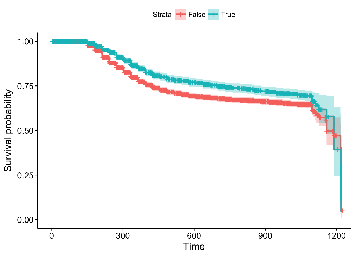
## Score (logrank) test = 3.22 on 1 df, p=0.07255You can see that the output is similar to previous model without stratification however, in this case, we do not have information about the hazard ratio of the stratification variable, IsBorrowerHomeowner. This variable is not really in the model. In any case, you can plot it…
ggsurvplot(survfit(m3), data = loan_filtered, conf.int = TRUE)