3.6 How to evaluate the PH assumption?
Now we are going to illustrate two methods to evaluate the proportional hazards assumptions: one graphical approach and one goodness-of-fit test. Recall that the Hazard Ratio that compares two specifications of the covariates (defined as \(\textbf{X}^*\) and \(\textbf{X}\)) can be expressed as
\[ HR = \exp(\sum_{j=1}^p \beta_j (X_j^* - X_j)) \] where \(\textbf{X}^*=(X_1^*, X_2^*, \ldots, X_j^*)\) and \(\textbf{X}=(X_1, X_2, \ldots, X_j)\), and proportionally of hazards assumption indicates that this quantity is constant over time. Equivalently, this means that the hazard for one individual is proportional to the hazard for any other individual, where the proportionality constant is independent of time.
Think about this…
It is important to note that if the graph of the hazards cross for two or more categories of a predictor of interest, the PH assumption is not met. However, althought the hazard functions do not cross, it is possible that the PH assumption is not met. Thus, rather than checking for crossing hazards, we need to use other apporaches.3.6.1 Graphical approach
The most popular graphical techniques for evaluating the PH assumption involves comparing estimated –ln(–ln) survival curves over different (combinations of) categories of variables being investigated.
A log–log survival curve is simply a transformation of an estimated survival curve that results from taking the natural log of an estimated survival probability twice.5
As we said, the hazard function can be rewritten as \[ S(t|\textbf X) = \bigg[ S_0(t) \bigg]^{e^{\sum_{j=1}^p \beta_j X_j}} \] and once we applied the -ln(-ln), the expression can be rewritten as \[ -\ln \bigg[-\ln S(t|\textbf X) \bigg] = - \sum_{j=1}^p \beta_j X_j - \ln \bigg[-\ln S_0(t|\textbf X) \bigg]. \]
Now, considering two different specifications of the covariates, corresponding to two different individuals, \(\textbf X_1\) and \(\textbf X_2\), and subtracting the second log–log curve from the first yields the expression
\[ -\ln \bigg[-\ln S(t|\textbf X_1) \bigg] = -\ln \bigg[-\ln S(t|\textbf X_2) \bigg] + \sum_{j=1}^p \beta_j (X_{1j} - X_{2j}) \]
This expression indicates that if we use a Cox model (well-used) and plot the estimated log-log survival curves for individuals on the same graph, the two plots would be approximately parallel. The distance between the two curves is the linear expression involving the differences in predictor values, which does not involve time.
Note that there is an important problem associated with this approach, that is, how to decide “how parallel is parallel?”. This fact can be subjective, thus the proposal is to be conservative for this decision by assuming the PH assumption is satisfied unless there is strong evidence of nonparallelism of the log–log curves.
Now we are going to check the proportinal hazards assumption for the variable IsBorrowerHomeowner. This can be done by plotting log-log Kaplan Meier survival estimates against time (or against the log of time) and evaluating whether the curves are reasonably parallel.
km_home <- survfit(Surv(time, status) ~ IsBorrowerHomeowner, data = loan_filtered)
#autoplot(km_home) # just to see the km curves

plot(km_home, fun = "cloglog", xlab = "Time (in days) using log",
ylab = "log-log survival", main = "log-log curves by clinic") 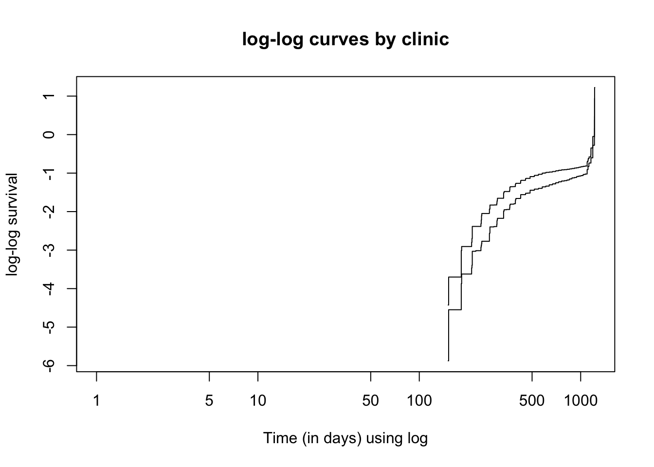
# another option
ggsurvplot(km_home, fun = "cloglog")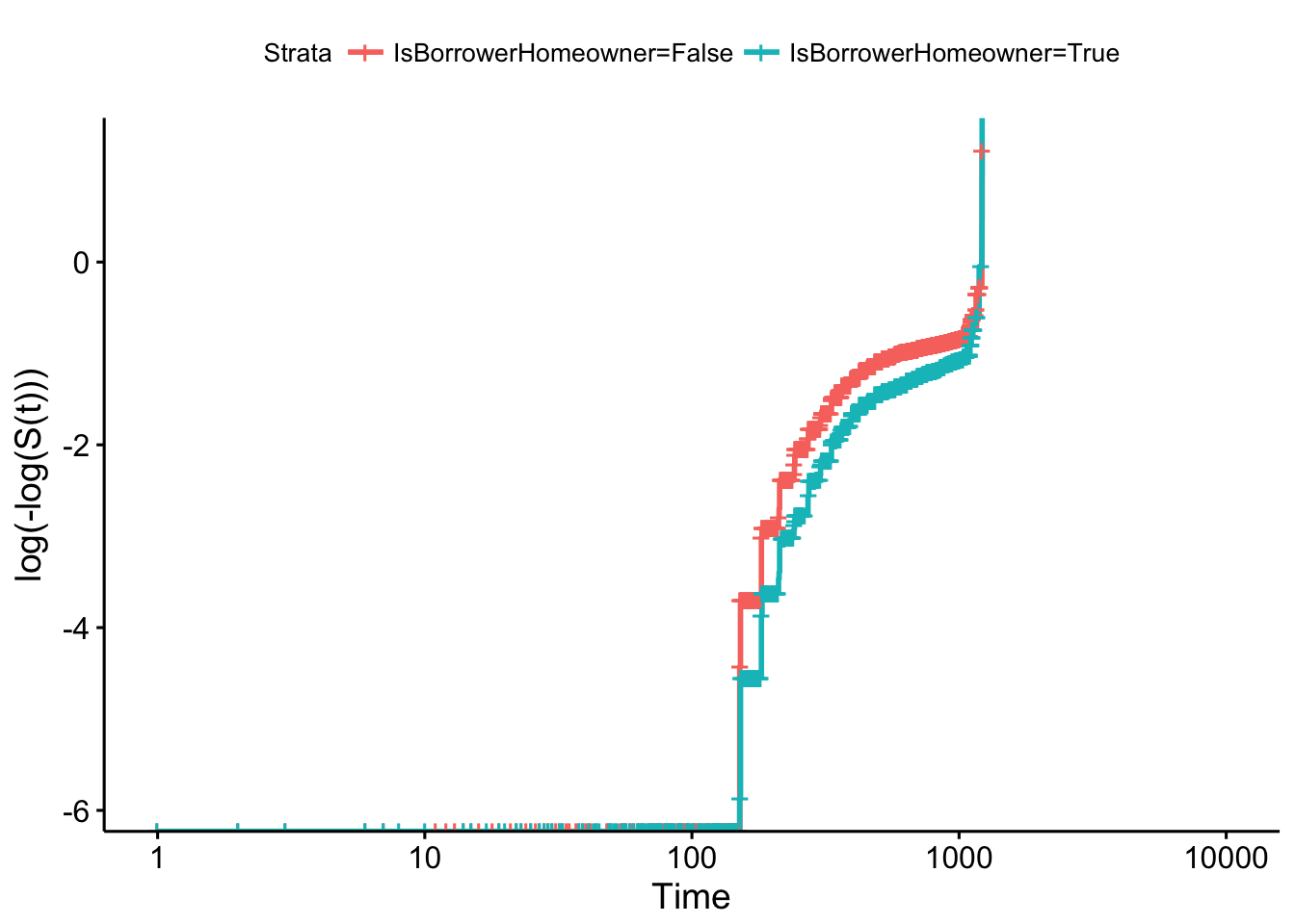
It seems that the proportional hazards assumption is violated as the log-log survival curves are not parallel.
Another graphical option could be to use the Schoenfeld residuals to examine model fit and detect outlying covariate values. Shoenfeld residuals represent the difference between the observed covariate and the expected given the risk set at that time. They should be flat, centered about zero. You can see the explanation in this paper.
The main idea is that he defined a partial residual as the different between the observed value of \(X_i\) and its conditional expectation given the risk set \(R_i\) and demostrated that these residuals have to be independent of the time. So, if you represent them ranked by its event time, this plot must not show any pattern.
ggcoxdiagnostics(m2, type = "schoenfeld")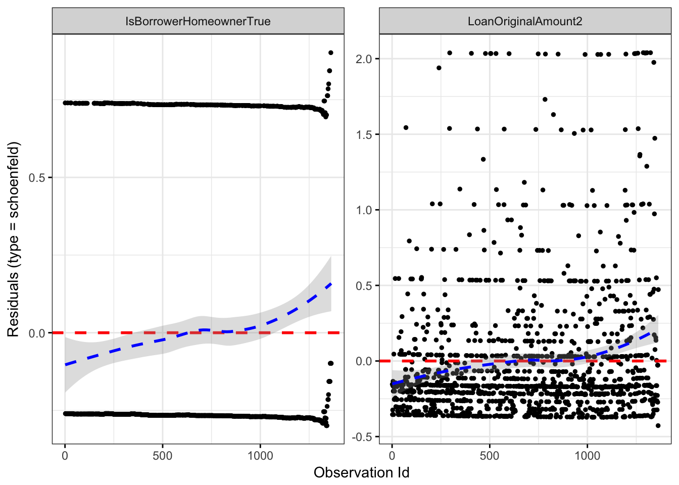
# another option
zph <- cox.zph(m2)
par(mfrow = c(1, 2))
plot(zph, var = 1)
plot(zph, var = 2)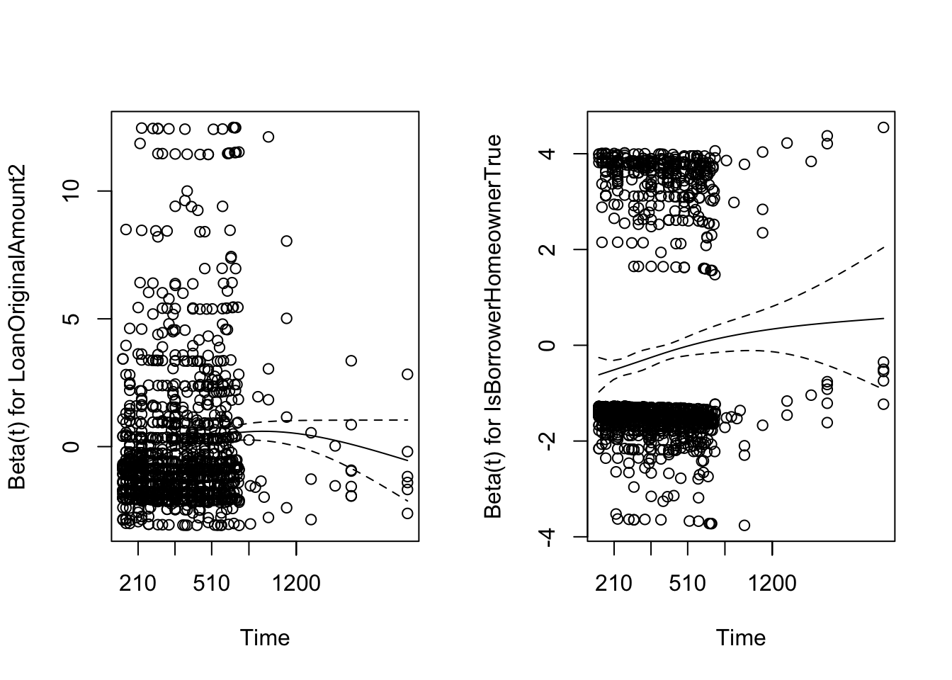
3.6.2 Goodness-of-fit test
A second approach for assessing the PH assumption involves goodness-of-fit (GOF) tests. To this end, different test have been proposed in the literature (Grambsch and Therneau 1994). We focuss in the Harrell (1986), a variation of a test originally proposed by Schoenfeld (1982). This is a test of correlation between the Schoenfeld residuals and survival time. A correlation of zero indicates that the model met the proportional hazards assumption (the null hypothesis).
This can be applied by means of the cox.zph function of the survival package.
cox.zph(m2)
##                           rho chisq        p
## LoanOriginalAmount2     0.130  27.1 1.96e-07
## IsBorrowerHomeownerTrue 0.103  14.0 1.81e-04
## GLOBAL                     NA  49.3 1.96e-11
It seems again that the proportional hazards assumption is not satisfied (as we saw with the log-log survival curves).
References
Grambsch, Patricia M., and Terry M. Therneau. 1994. “Proportional Hazards Tests and Diagnostics Based on Weighted Residuals.” Biometrika 81 (3). Oxford University Press: 515–26. doi:10.1093/biomet/81.3.515.
Harrell, F. 1986. “The Phglm Procedure.” In SAS Supplemental Library User’s Guide, Version 5. Cary, NC: SAS Institute Inc.
Schoenfeld, David. 1982. “Partial Residuals for the Proportional Hazards Regression Model.” Biometrika 69 (1): 239–41. doi:10.1093/biomet/69.1.239.
Note that the scale of the y-axis of an estimated survival curve ranges between 0 and 1, whereas the corresponding scale for a -ln(-ln) curve ranges between \(-\infty\) and \(+\infty\).↩