Deep learning
Learning outcomes/objective:
- Discuss a few things about the term paper.
- Shortly discuss stratified splitting & class imbalance
- Quickly repeat various pre-processing steps (motivation, types).
- Learn…
- …about the basic concepts used to describe deep learning models (e.g., layers).
- …how to use deep learning with tidymodels (a simple example!).
Source(s): The material for the following sessions is mainly based the excellent book Chollet and Allaire (2018); Classification models using a neural network
1 Fundstücke/Finding(s)
2 Term paper discussions & recommendations
- Make sure to read chapters corresponding to methods (e.g., random forests)
- Theory part in paper = part where you discuss various possible important features (but not necessarily all)
- When comparing models (e.g., linear regression vs. random forest)
- Same split (training/test) for both so that ultimate accuracy evaluation is on the same test data
- Steps inbetween (preprocessing = recipes, cross-validation, etc.) may differ
- Define different workflows for each model that you compare
- Quarto: https://osf.io/ur4xn
- Introduction: https://quarto.org/docs/get-started/hello/rstudio.html
3 Why preprocess data and how?
3.1 Why preprocess data and how? (1)
- Tidymodels allows for using recipes to preprocess data (e.g, normalization, centering etc.)
- Why?
- Improved model performance: can help to make features more compatible with ML algorithms increasing their accuracy/efficiency
- e.g., ML algorithms typically require numerical inputs, hence, we use techniques like one-hot encoding, label encoding, or ordinal encoding to convert categorical variables into numerical representations
- Facilitated interpretation: pre-processing may facilitate the interpretation of modelling results
- e.g., centering can make it easier to interpret the regression coefficients as they represent the average effect when all other variables are held constant
- Handling algorithm requirements: some machine learning algorithms may have assumptions or requirements related to the scale or format of the input features
- e.g., standardization of features for ridge regression so that penalty term is not influenced by predictor scales
- Improved model performance: can help to make features more compatible with ML algorithms increasing their accuracy/efficiency
3.2 Recipes: Why preprocess data and how? (2)
- Handling missing data:
step_impute_*()(e.g., see here for substituting missing values of numeric variables by the training set median of those variables) - Encoding categorical variables (reference):
step_dummy()(see alsoone_hot = TRUE) as described here- e.g., because ML algorithms typically want numeric input
- Scaling and normalization (reference):
step_center()to center numeric data;step_normalize()to center and scale numeric data;step_range()to scale numeric data to a specific range;step_scale()to scale numeric data- e.g., scaling to common range or normalizing to mean zero and unit variance
- e.g., because some algorithms are sensitive to differences in feature scales, scaling prevents features from dominating model (improves stability and convergence of algorithms)
- …others such as feature selection and dimensionality reduction (reference;
step_pca()for PCA Signal Extraction), outlier detection and removal and feature engineering (e.g.,step_poly()creates new columns that are basis expansions of variables using orthogonal polynomials)
3.3 When does it make sense to transform the outcome variable?
- Be careful: assess the benefits, potential implications, and interpretability trade-offs before applying any transformation to the outcome variable
- Transforming the outcome variable in a machine learning model can make sense in the following situations:
- a transformation (e.g., logarithmic) can help normalize a skewed distribution and can improve a model’s performance (e.g., fulfilling assumptions)
- Homoscedasticity: a transformation can help stabilize the variance and achieve more consistent residual errors across different predicted values (e.g., linear models)
- Linearity: transforming the outcome variable can help achieve linearity (better for linear models!)
- Outlier or extreme value mitigation: Transforming the outcome variable can reduce the influence of outliers or extreme values, making the model more robust.
- Interpretability: Transforming the outcome variable can aid in interpretability, e.g., logarithmic transformations can allow the coefficients in the model to be directly interpreted as percentage changes (e.g., predicting growth)
4 Deep learning
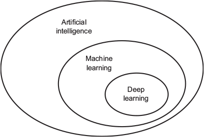
4.1 Artificial, machine and deep learning
- Artificial intelligence: The effort to automate intellectual tasks normally performed by humans (Chollet’s concise definition, field born in 1950s, Symbolic AI → Machine learning)
- Machine learning: See [Machine learning as programming paradigm]
- Deep learning: …see next slides!
4.2 Classical ML: What it does (1)
- Difference between ML and Deep Learning
- Classical ML: We need three things
- Input data points (e.g., sound files of people speaking, images)
- Examples of the expected output (e.g., human-generated transcripts of sound files, tags for images such as “dog,” “cat,” etc.)
- Could be binary, categorical or continuous variable
- A way to measure whether the algorithm (model!) is doing a good job
- e.g., training error rate
- Necessary to evaluate algorithm’s (model’s!) current output and its expected output
- Measurement = feedback signal to adjust algoritm (model!) → adjustment step is what we call learning
- Manual adjustment in [Lab: Resampling & cross-validation]
- ML model: transforms input data into meaningful outputs, a process that is “learned” from exposure to known examples of inputs and outputs
- Central problem in ML (and deep learning): Learn useful representations of the input data at hand – representations that get us closer to the expected output (“Representations”1)
- Further reading.. Chollet and Allaire (2018, Ch. 1.1.3)
4.3 Classical ML: What it does (2)
- All ML algorithms/models: Automatically find transformations that turn data into more-useful representations for a given task (e.g., coordinate changes or linear projections)
- ML (technically): searching for useful representations of some input data, within a predefined space of possibilities, using guidance from a feedback signal
- Classic ML algorithms (e.g., logistic regression): usually not creative in finding transformations; they just search through predefined set of operations, called a hypothesis space
- So what is deep learning? Why is it special?2
4.4 The ‘deep’ in deep learning (1)
- Deep learning (DL) = mathematical framework = subfield of machine learning
- New take on learning representations from data that puts an emphasis on learning successive layers of increasingly meaningful representations
- “deep” stands for this idea of successive layers of representations
- Depth of model = how many layers contribute to a model of the data
- Modern deep learning often involves tens or even hundreds of successive layers of representations
- Layered representations are (almost always) learned via models called neural networks (structured in literal layers stacked on top of each other)
- “Neural network”
- Reference to neurobiology as central DL concepts inspired from understanding brain
- BUT no evidence that brain implements mechanisms used in DL!
4.5 The ‘deep’ in deep learning (2)
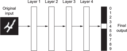
- What do the representations learned by a deep-learning algorithm look like?
- Let’s examine how a network several layers deep (see Figure 2) transforms an image of a digit in order to recognize what digit it is.
- Graph below: visualizes how an image showing “4” is transformed into the number 4
4.6 The ‘deep’ in deep learning (3)
- Q: What is illustrated in Figure 3?
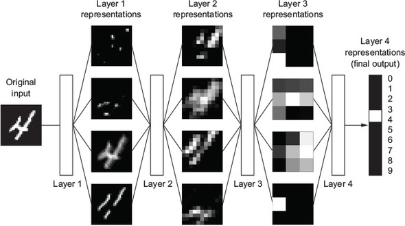
Answer
- Network transforms the digit image into representations that are…
- increasingly different from the original image (going from layer to layer)
- increasingly informative about the final result
- Deep network = multistage information-distillation operation
- Information goes through successive filters and comes out increasingly purified (that is, useful with regard to some task)
- Deep learning (technically): a multistage way to learn data representations
4.7 Understanding how DL works (1)
- Reminder: ML about mapping inputs (e.g., images) to targets/outputs (e.g., label “cat”).. through observing many examples of inputs and targets/outputs
- Neural networks: do this input-to-target mapping via a deep sequence of simple data transformations (layers) [data transformations are learned by exposure to examples]
- But how does this happen concretely? See Figure 4.
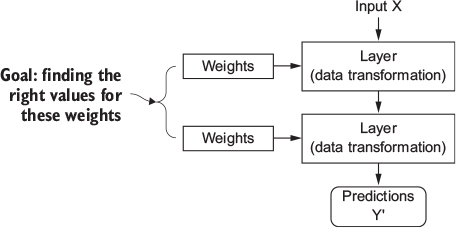
- Specification of what a layer does to its input data is stored in the layer’s weights (= a bunch of numbers) (see Figure 4)
- Weights are also sometimes called the parameters of a layer
- Learning (in this context): Find set of values for the weights of all layers in a network, such that the network will correctly map example inputs to their associated targets
- Deep neural network can contain tens of millions of parameters
- Finding correct values for all of them may seem like a daunting task…
4.8 Understanding how DL works (2)
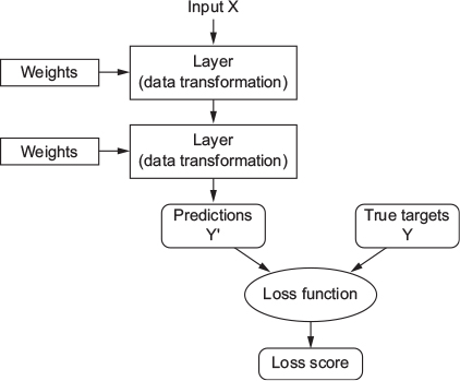
- Loss function (also called objective function)
- To control output of neural network, you need to be able to measure how far this output is from what you expected
- Loss function takes predictions of the network and the true target (what you wanted the network to output) and computes a distance score, capturing how well the network has done on this specific example (see Figure 5).
4.9 Understanding how DL works (3)
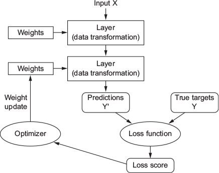
- Loss score: Is used as feedback signal to adjust the value of the weights, in a direction that will lower loss score for the current example (see Figure 6)
- Adjustment = job of optimizer
- Optimizer: Implements Backpropagation algorithm (central algorithm in deep learning)
- Starting point: weights of the network are assigned random values and network implements series of random transformations
- Output far from targets and loss score is high
- Network processes examples and adjusts weights a little in correct direction → with every example loss score decreases (= training loop)
- Training loop: repeated a sufficient number of times, yields weight values that minimize the loss function
- Typically tens of iterations over thousands of examples
- Training loop: repeated a sufficient number of times, yields weight values that minimize the loss function
- Starting point: weights of the network are assigned random values and network implements series of random transformations
- Trained network: Network with minimal loss for which the outputs are as close as they can be to the targets
4.10 Achievements of deep learning
- DL achieved nothing short of a revolution in the (ML) field
- Remarkable results: Perceptual problems (seeing, hearing) that have long been elusive for machines
- Near-human-level image classification; Near-human-level speech recognition; Near-human-level handwriting transcription; Improved machine translation; Improved text-to-speech conversion; Digital assistants such as Google Now and Amazon Alexa; Near-human-level autonomous driving; Improved ad targeting, as used by Google, Baidu, and Bing; Improved search results on the web; Ability to answer natural-language questions; Superhuman Go playing
- Still exploring full extent of what DL can do
- Applications outside of machine perception/natural-language understanding, such as formal reasoning -> may assist humans in science, software development and more
- ML and causal thinking
- “The key [Pearl] […] argues, is to replace reasoning by association with causal reasoning. Instead of the mere ability to correlate fever and malaria, machines need the capacity to reason that malaria causes fever. Once this kind of causal framework is in place, it becomes possible for machines to ask counterfactual questions — to inquire how the causal relationships would change given some kind of intervention — which Pearl views as the cornerstone of scientific thought.”
4.11 Short-term hype & promise of AI (Ch. 1.1.7, 1.1.8)
- Chollet and Allaire (2018): Some world-changing applications within reach but many more likely to remain elusive for a long time
- e.g., autonomous cars vs. believable dialogue systems, human-level machine translation across arbitrary languages, and human-level natural-language understanding
- …talk of human-level general intelligence shouldn’t be taken too seriously
- Past hype cycles: Symbolic AI in 1960s; Expert system in 1980s; now third hype cycle of AI?
- Promise of AI:
- Think of the applications you use.. but your doctor, accountant etc. does not use it yet
- AI has yet to transition to being central to the way we work, think, and live
- “Don’t believe the short-term hype, but do believe in the long-term vision” (Chollet and Allaire 2018, Ch. 1.1.8)
4.12 The universal workflow of machine learning
- Defining the problem and assemble a dataset (Chollet and Allaire 2018, Ch. 4.5)
- Define the problem at hand and the data on which we’ll train. Collect this data, potentially annotate with labels (supervised learning)
- Choose a measure of success
- Choose how we’ll measure success on your problem. Which metrics will you monitor on our validation data?
- Deciding on an evaluation protocol
- Determine our evaluation protocol: Hold-out validation? K-fold validation? Which portion of the data should we use for validation?
- Prepare our data
- Developing a model that does better than a baseline (baseline?)
- Scaling up: developing a model that overfits
- Regularize our model and tune our hyperparameters based on performance on the validation data
- A lot of machine-learning research tends to focus only on this step-but keep the big picture in mind
4.13 Getting started: Network anatomy
- Training a neural network revolves around the following objects (see Figure 7, Chollet and Allaire (2018), Ch. 3)
- Layers, which are combined into a network (or model)
- The input data and corresponding targets
- The loss function, which defines the feedback signal used for learning
- The optimizer, which determines how learning proceeds.
4.14 Layers: the building blocks of deep learning
- Deep-learning model: directed, acyclic graph of layers
- Most common is a linear stack of layers, mapping a single input to a single output
- Layer: a data-processing module that takes as input 1+ tensors (e.g. vectors) and that outputs one or more tensors
- Different layer types for different tensor formats/data processing types (e.g., densely connected layers, recurrent layers etc.)
- Layer’s state: the layer’s weights which together contain the network’s knowledge
- Layers = LEGO bricks of deep learning (this metaphor is made explicit by frameworks like Keras)
- Building deep-learning models in Keras: Clip together compatible layers to form useful data-transformation pipelines
- Layer compatibility = every layer will only accept input tensors of a certain shape and will return output tensors of a certain shape
- Keras takes care of layer compatibility (dynamically built to match shape of incoming layer)
# Example code for keras DL model
# Network architecture
  model <- keras_model_sequential() %>% # linear stack of layers
    layer_dense(units = 64, # Output space dim.
                activation = "relu", # Activation function (linear)
                input_shape = dim(train_data)[[2]]) %>% # Input Dim.
    layer_dense(units = 64,
                activation = "relu") %>%
    layer_dense(units = 1)

# "relu": Rectified linear unit activation function
4.15 Loss functions and optimizers
- Once network architecture (
model) is defined → choose loss function & optimizer - Loss function (also called objective function)
- Quantity that will be minimized during training (measure of success)
- Optimizer
- Determines how the network will be updated based on the loss function
# Example code for keras DL model: Compile the model
model %>% compile(
    optimizer = "rmsprop", # Optimizer algorithm
    loss = "mse", # Mean squared error loss function
    metrics = c("mae") # mean absolute error (MAE)
  )
4.16 Keras & R packages
- Keras: deep-learning framework that provides a convenient way to define and train almost any kind of deep-learning model
- Initially developed for researchers, with aim of enabling fast experimentation
- Used by over 150,000 users (researchers, engineers, etc.)
- Used at Google, Netflix, Uber, CERN, Yelp, Square, and hundreds of startups
- Keras is also a popular framework on Kaggle
keras: R package that provides the R interface to Kerastensorflow: R package that provides interface with Tensorflow- TensorFlow: open source software library for numerical computation using data flow graphs (originally developed by researchers and engineers working on the Google Brain Team)
- Alternatives: Pytorch (see discussion here)
5 Lab: Deep learning (new)
Below we will discuss a very short example of how we can setup a deep learning model using tidymodels (based on Classification models using a neural network).
5.1 Installation: Keras & tensorflow
Keras and Tensorflow can be installed relatively simply from within R/Rstudio. Python is running in the background and at some point (if it’s not installed already) you will be asked “Would you like to download and install Miniconda?”. Simply answer “Y”.
# Install Keras
install.packages("keras")
# Check if it works
library(keras)

# If not python installed install this as well
  # No non-system installation of Python could be found.
  # Would you like to download and install Miniconda?
  # Would you like to install Miniconda? [Y/n]: Y -> YES!

# Check tensorflow installation (if not install)
  # tensorflow::install_tensorflow()
library(tensorflow)

# Restart R/Rstudio
Restart R studio after the installation!
# install.packages(pacman)
# https://tensorflow.rstudio.com/install/
pacman::p_load(tidyverse,
               tidymodels,
               naniar,
               keras,
               tensorflow)
5.2 The data
Our lab is based on Lee, Du, and Guerzhoy (2020) and on James et al. (2013, chap. 4.6.2) with various modifications. We will be using the dataset at LINK that is described by Angwin et al. (2016). - It’s data based on the COMPAS risk assessment tools (RAT). RATs are increasingly being used to assess a criminal defendant’s probability of re-offending. While COMPAS seemingly uses a larger number of features/variables for the prediction, Dressel and Farid (2018) showed that a model that includes only a defendant’s sex, age, and number of priors (prior offences) can be used to arrive at predictions of equivalent quality.
We first import the data into R:
data <- read_csv(sprintf("https://docs.google.com/uc?id=%s&export=download",
                         "1plUxvMIoieEcCZXkBpj4Bxw1rDwa27tj"))
Then we create a factor version of is_recid that we label (so that we can look up what is what aftewards). We also order our variabels differently.
data <- data %>% select(-id, -name)
data$is_recid_factor <- factor(data$is_recid,
                        levels = c(0,1),
                        labels = c("no", "yes"))
data <- data %>% select(compas_screening_date, is_recid,
                        is_recid_factor, age, priors_count, everything())
We have previously explored this dataset here.
5.3 Splitting the datasets
Below we split the data into training data and test data (Split 1). Then we further split (Split 2) the training data into an analysis dataset (sometimes also called training data) and an assessment dataset (often called validation set) (Kuhn and Johnson 2019). This is illustrated in Figure 8. We often call splits of the second kind folds. Below we have only one fold corresponding to “Resample 1” in Figure 8.

# Split the data into training and test data
  data_split <- initial_split(data, prop = 0.80)
  data_split # Inspect
<Training/Testing/Total>
<5771/1443/7214># Extract the two datasets
data_train <- training(data_split)
data_test <- testing(data_split) # Do not touch until the end!
dim(data_train)[1] 5771 52 dim(data_test)[1] 1443 52# Further split the training data into analysis (training2) and assessment (validation) dataset
data_folds <- validation_split(data_train, prop = .80)
# Extract analysis ("training data 2") and assessment (validation) data
data_analysis <- analysis(data_folds$splits[[1]])
data_assessment <- assessment(data_folds$splits[[1]])
dim(data_analysis)[1] 4616 52 dim(data_assessment)[1] 1155 525.4 The outcome
We can also try to visualize the outcome as a function of features. Below we visualize recidivism as a function of age and the number of prior offenses (Q: What we would be a better way to visualize this data?).
ggplot(data_train,
       aes(x = age,
           y = priors_count,
           col = is_recid_factor)) +
  geom_point(alpha = .2)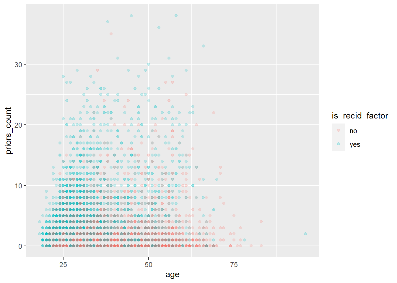
5.5 Specifying, fitting and evaluating the model
In our short code example we will use a single hidden layer neural network to predict the outcome recidivism. Beforehand, we transform the predictor columns to be more symmetric (via the step_BoxCox() function) and on a common scale (using step_normalize()). We use a recipe to define these transformations:
model_recipe <-
  recipe(is_recid_factor ~ age + priors_count + race, data = data_train) %>%
  step_dummy(all_nominal_predictors()) %>%
  step_BoxCox(all_predictors()) %>%
  step_normalize(all_predictors())
Then, we can use the keras package to specify a model/workflow with 10 hidden units and a 10% dropout rate, to regularize the model:
set.seed(57974)

# Specify model
model_nnet <-
  mlp(epochs = 100, hidden_units = 10, dropout = 0.1) %>%
  set_mode("classification") %>%
  # Also set engine-specific `verbose` argument to prevent logging the results:
  set_engine("keras", verbose = 0)


# Specify workflow
wflow_nnet <-
  workflow() %>%
  add_recipe(model_recipe) %>%
  add_model(model_nnet)
Then we can fit the model to data_analysis and evaluate it using data_assessment.
# Fit/train the model
fit_nnet <- wflow_nnet %>%
  fit(data = data_analysis)

fit_nnet
== Workflow [trained] ==========================================================
Preprocessor: Recipe
Model: mlp()
-- Preprocessor ----------------------------------------------------------------
3 Recipe Steps
* step_dummy()
* step_BoxCox()
* step_normalize()
-- Model -----------------------------------------------------------------------
Model: "sequential"
________________________________________________________________________________
Layer (type) Output Shape Param #
================================================================================
dense (Dense) (None, 10) 80
dense_1 (Dense) (None, 10) 110
dropout (Dropout) (None, 10) 0
dense_2 (Dense) (None, 2) 22
================================================================================
Total params: 212
Trainable params: 212
Non-trainable params: 0
________________________________________________________________________________# Add predictions to data_assments
data_assessment <- data_assessment %>%
bind_cols( # add predictions as columns
predict(fit_nnet, new_data = data_assessment),
predict(fit_nnet, new_data = data_assessment, type = "prob")
) %>%
select(age, priors_count, race,
is_recid_factor, .pred_class, .pred_no,
.pred_yes)
data_assessment# A tibble: 1,155 x 7
age priors_count race is_recid_factor .pred_c~1 .pred~2 .pred~3
<dbl> <dbl> <chr> <fct> <fct> <dbl> <dbl>
1 20 0 Hispanic yes yes 0.379 0.621
2 45 0 Hispanic no no 0.915 0.0852
3 57 1 Hispanic no no 0.912 0.0879
4 20 1 African-American yes yes 0.115 0.885
5 25 1 African-American yes no 0.565 0.435
6 34 2 African-American yes no 0.755 0.245
7 23 0 African-American yes no 0.681 0.319
8 22 0 African-American yes no 0.570 0.430
9 65 0 African-American no no 0.904 0.0956
10 48 0 Caucasian no no 0.898 0.102
# ... with 1,145 more rows, and abbreviated variable names 1: .pred_class,
# 2: .pred_no, 3: .pred_yes# Check accuracy in assessment data
data_assessment %>% accuracy(truth = is_recid_factor, estimate = .pred_class)# A tibble: 1 x 3
.metric .estimator .estimate
<chr> <chr> <dbl>
1 accuracy binary 0.683 data_assessment %>% roc_auc(truth = is_recid_factor, estimate = .pred_no)# A tibble: 1 x 3
.metric .estimator .estimate
<chr> <chr> <dbl>
1 roc_auc binary 0.737 data_assessment %>% conf_mat(truth = is_recid_factor, estimate = .pred_class) Truth
Prediction no yes
no 442 198
yes 168 347Subsequently, we would change our model in various ways (e.g., the number of hidden units, features etc.) and reassess it using data_assessment (importantly, we can also use resampling instead of a single split into data_analysis and data_assessment).
Once we are happy with the model we can train it using the the whole training dataset data_train and assess the accuracy using data_test.
# Fit/train the model
fit_nnet <- wflow_nnet %>%
  fit(data = data_train)

# Add predictions to data_test
data_test <- data_test %>%
  bind_cols( # add predictions as columns
    predict(fit_nnet, new_data = data_test),
    predict(fit_nnet, new_data = data_test, type = "prob")
  ) %>%
  select(age, priors_count, race,
         is_recid_factor, .pred_class, .pred_no,
         .pred_yes)
data_test
# A tibble: 1,443 x 7
age priors_count race is_recid_factor .pred_c~1 .pred~2 .pred~3
<dbl> <dbl> <chr> <fct> <fct> <dbl> <dbl>
1 69 0 Other no no 0.929 0.0710
2 31 7 African-American yes yes 0.123 0.877
3 37 0 Hispanic no no 0.912 0.0879
4 31 5 Caucasian yes yes 0.245 0.755
5 24 1 Hispanic yes no 0.567 0.433
6 26 5 African-American yes yes 0.0808 0.919
7 33 0 African-American yes no 0.891 0.109
8 51 2 African-American no no 0.863 0.137
9 63 1 Hispanic no no 0.916 0.0838
10 30 0 Hispanic no no 0.896 0.104
# ... with 1,433 more rows, and abbreviated variable names 1: .pred_class,
# 2: .pred_no, 3: .pred_yes# Check accuracy in assessment data
data_test %>% accuracy(truth = is_recid_factor, estimate = .pred_class)# A tibble: 1 x 3
.metric .estimator .estimate
<chr> <chr> <dbl>
1 accuracy binary 0.682 data_test %>% roc_auc(truth = is_recid_factor, estimate = .pred_no)# A tibble: 1 x 3
.metric .estimator .estimate
<chr> <chr> <dbl>
1 roc_auc binary 0.742 data_test %>% conf_mat(truth = is_recid_factor, estimate = .pred_class) Truth
Prediction no yes
no 541 246
yes 213 4436 All the code
labs = knitr::all_labels()
ignore_chunks <- labs[str_detect(labs, "exclude|setup|solution|get-labels")]
labs = setdiff(labs, ignore_chunks)
References
Angwin, Julia, Jeff Larson, Lauren Kirchner, and Surya Mattu. 2016. “Machine Bias.” https://www.propublica.org/article/machine-bias-risk-assessments-in-criminal-sentencing.
Chollet, Francois, and J J Allaire. 2018. Deep Learning with R. 1st ed. Manning Publications.
Dressel, Julia, and Hany Farid. 2018. “The Accuracy, Fairness, and Limits of Predicting Recidivism.” Sci Adv 4 (1): eaao5580.
James, Gareth, Daniela Witten, Trevor Hastie, and Robert Tibshirani. 2013. An Introduction to Statistical Learning: With Applications in R. Springer Texts in Statistics. Springer.
Kuhn, Max, and Kjell Johnson. 2019. Feature Engineering and Selection: A Practical Approach for Predictive Models. CRC press (Taylor & Francis).
Lee, Claire S, Jeremy Du, and Michael Guerzhoy. 2020. “Auditing the COMPAS Recidivism Risk Assessment Tool: Predictive Modelling and Algorithmic Fairness in CS1.” In Proceedings of the 2020 ACM Conference on Innovation and Technology in Computer Science Education, 535–36. ITiCSE ’20. New York, NY, USA: Association for Computing Machinery.
Footnotes
What’s a representation? A different way to look at data (to represent or encode data); e.g., color image encoded in RGB format (red-green-blue) or in the HSV format (hue-saturation-value): these are two different representations of the same data; Some (classification) tasks that may be difficult with one representation can become easy with another (e.g, “select all red pixels in the image” simpler in RGB than HSV)↩︎