| Predicted values | ||
|---|---|---|
| 0 | 1 | |
| True values | ||
| 0 | 540 | 224 |
| 1 | 255 | 424 |
Measurement and assessment of accuracy
Learning outcomes/objective: Learn/understand…
- …further concepts concerning model accuracy (precision, recall, etc.).
- …bias-variance trade-off.
1 Fundstücke/Finding(s)
- There is a new pipe..
|>instead of%>%(e.g., blog post)|>does not rely onmagrittrpackage
- Is the glass half empty or half full?
- How AI experts are using GPT-4: Can anyone do a presentation on GPT-4 and the paper below? (functioning, use-cases)
- GPTs are GPTs: An Early Look at the Labor Market Impact Potential of Large Language Models
- See Table 11, page 30
2 Bias-variance trade-off
- See James et al. (2013, Ch. 2.2.2)
2.1 Bias-variance trade-off (1)
- James et al. (2013) introduce bias-variance trade-off before turning to classification
- What do we mean by the variance and bias of a statistical learning method? (James et al. 2013, Ch. 2.2.2)
- Variance refers to amount by which \(\hat{f}\) would change if estimated using a different training data set
- Ideally estimate for \(f\) should not vary too much between training sets
- If method has high variance then small changes in training data can result in large changes in \(\hat{f}\)
- More flexible methods/models usually have higher variance
- Bias refers to the error that is introduced by approximating a (potentially complicated) real-life problem (=\(f\)) through a much simpler model
- e.g., linear regression assumes linear relationship between \(Y\) and \(X_{1},X_{2},...,X_{p}\) but unlikely that real-life problems truly have linear relationship producing bias/error
- e.g., predict income \(Y\) with age \(X\)
- If true \(f\) is substantially non-linear, linear regression will not produce accurate estimate \(\hat{f}\) of \(f\), no matter how many training observations,
- Variance refers to amount by which \(\hat{f}\) would change if estimated using a different training data set
2.2 Bias-variance trade-off (2)
Bias error: error from erroneous assumptions in the learning algorithm
- High bias can cause an algorithm to miss relevant relations between features and target outputs (underfitting)
Variance: error from sensitivity to small fluctuations in the training set
- High variance may result from an algorithm modeling the random noise in the training data (overfitting)
Bias-variance trade-off: Property of model that variance of parameter(s) estimated across samples can be reduced by increasing the bias in the estimated parameters
Bias-variance dilemma/problem: Trying to simultaneously minimize these two sources of error that prevent supervised learning algorithms from generalizing beyond their training set
2.3 Bias-variance trade-off (3)
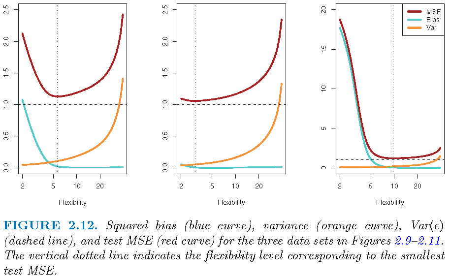
- “General rule”: with more flexible methods, variance will increase and bias will decrease
- Relative rate of change of these two quantities determines whether test MSE (regression problem) increases or decreases
- As we increase flexibility of a class of methods, bias tends to initially decrease faster than the variance increases
- Consequently, the expected test MSE declines as shown in Figure 1.
- Q: What does Figure 1 illustrate and which level of flexibility would be desirable?
2.4 Bias-variance trade-off (4)
- Good test set performance requires low variance as well as low squared bias
- Trade-off because easy to obtain method with…
- …extremely low bias but high variance
- e.g., just draw a curve that passes through every single training observation
- …very low variance but high bias
- e.g., by fitting a horizontal line to the data
- …extremely low bias but high variance
- Trade-off because easy to obtain method with…
- Challenge lies in finding a method for which both the variance and the squared bias are low
- This idea will return throughout the semester!
- In real-life situation \(f\) is unobserved hence not possible to compute test MSE, bias, or variance for a statistical learning method (because we fit our model to the training data not the test data!)
- But good to keep in mind and later on we discuss methods to estimate test MSE using training (cross-validation!)
3 Exercise 1
Adapted from James et al. (2013, Exercise 2.4.1): Thinking of our classification problem (predicting recidivism), indicate whether we would generally expect the performance of a flexible statistical learning method to be better or worse than an inflexible method. Justify your answer.
- The sample size \(n\) is extremely large, and the number of predictors \(p\) is small.
- The number of predictors \(p\) is extremely large, and the number of observations \(n\) is small.
- The relationship between the predictors and response is highly non-linear.
- The variance of the error terms, i.e. \(\sigma^{2}=Var(\epsilon)\), is extremely high.
4 Exercise 2
James et al. (2013, Exercise 2.4.2): Explain whether each scenario is a classification or regression problem, and indicate whether we are most interested in inference or prediction. Finally, provide \(n\) and \(p\).
- We collect a set of data on the top 500 firms in the US. For each firm we record profit, number of employees, industry and the CEO salary. We are interested in understanding which factors affect CEO salary.
- We are considering launching a new product and wish to know whether it will be a success or a failure. We collect data on 20 similar products that were previously launched. For each product we have recorded whether it was a success or failure, price charged for the product, marketing budget, competition price, and ten other variables.
- We are interesting in predicting the % change in the US dollar in relation to the weekly changes in the world stock markets. Hence we collect weekly data for all of 2012. For each week we record the % change in the dollar, the % change in the US market, the % change in the British market, and the % change in the German market.
5 Assessing classification error
- See James et al. (2013, Ch. 4.4.3)
5.1 True/false negatives/positives
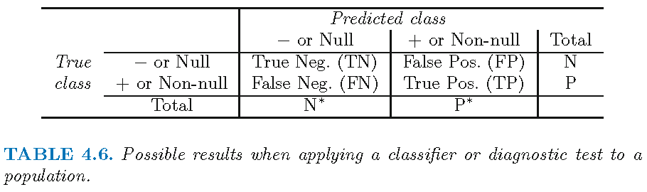
- Q: What does Figure 2 (a table!) illustrate? What do we find in the different cells?
5.2 Precision and recall (binary classification)
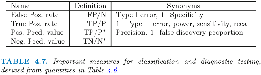
- Precision \((TP/P^{*})\)
- Number of true positive (TP) results divided by the number of all positive results (P*), including those not identified correctly
- e.g., N of patients that have cancer AND are predicted to have cancer (true positives TP) DIVIDED by N of all patients predicted to have cancer (positives P*).
- Recall \((TP/P)\)
- Number of true positive results divided by the number of all samples that should have been identified as positive (P)
- e.g., N of patients that have cancer AND are predicted to have cancer (true positives TP) DIVIDED by N of all patients that have cancer and SHOULD have been predicted to have cancer (the “trues” P).
6 Exercise: recidivism
- Take our recidivism example where reoffend = recidivate = 1 = positive and not reoffend = not recidivate = 0 and discuss the table in Figure 2 using this example.
- Take our recidivism example and discuss the different definitions (Column 2) in the Table in Figure 3. Explain what precision and recall would be in that case.
Answer
Precision \((TP/P^{*})\): N of prisoners that recidivate AND are predicted to recidivate (true positives TP) DIVIDED by N of all prisoners predicted to recidivate
Recall \((TP/P)\): N of prisoners that recidivate AND are predicted to recidivate (true positives TP) DIVIDED by N of all prisoners that recidivate and SHOULD have been predicted to recidivate (the “trues” P).
7 Exercise: Calculate precision and recall
- Below you find the table cross-tabulating the true values (rows) with the predicted values (columns) calculated in ?@sec-accuracy-test-data-error for the test data.
7.1 F-1 score
- Source: https://en.wikipedia.org/wiki/F-score
- F-score or F-measure is a measure of a test’s accuracy
- is the harmonic mean of precision and recall
- represents both precision and recall in one metric (one could also weight one or the other higher)
- Highest possible value of an F-score is 1.0, indicating perfect precision and recall, and the lowest possible value is 0, if either precision or recall are zero
- \({\displaystyle F_{1}={\frac {2}{\mathrm {recall} ^{-1}+\mathrm {precision} ^{-1}}}=2{\frac {\mathrm {precision} \cdot \mathrm {recall} }{\mathrm {precision} +\mathrm {recall} }}={\frac {2\mathrm {tp} }{2\mathrm {tp} +\mathrm {fp} +\mathrm {fn} }}}\)
- Q: What is the F1-score for the data in Table 1?
8 Error rates and ROC curve (binary classification)
- See James et al. (2013, Ch. 4.4.3)
- The error rates are a function of the classification threshold
- If we lower the classification threshold (e.g., use a predicted probability of 0.3 to classify someone as reoffender) we classify more items as positive (e.g. predict them to recidivate), thus increasing both False Positives and True Positives
- See James et al. (2013), Fig 4.7, p. 147
- Goal: we want to know how error rates develop as a function of the classification threshold
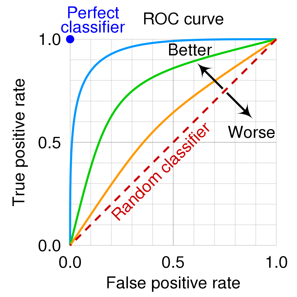
- The ROC curve is a popular graphic for simultaneously displaying the two types of errors (false positives, true positives rate) for all possible thresholds
- See James et al. (2013), Fig 4.8, p. 148 where \(1 - specificity = FP/N = \text{false positives rate (FPR)}\) and \(sensitivity = TP/P = \text{true positives rate (TPR)}\)
- The Area under the (ROC) curve (AUC) provides the overall performance of a classifier, summarized over all possible threshold (James et al. 2013, 147)
- The maximum is 1, hence, values closer to it a preferable as shown in Figure 4
References
James, Gareth, Daniela Witten, Trevor Hastie, and Robert Tibshirani. 2013. An Introduction to Statistical Learning: With Applications in R. Springer Texts in Statistics. Springer.