Lab: Extracting predicted values and model stats

Learning outcomes/objective - Learn how to extract model predictions in R

1 Packages

  • broom package (see ?function for arguments)
    • tidy(): Returns statistical findings of models (e.g., coefficients + stats)
    • glance(): Returns one-row summary of model (e.g., R-squared as measure of fit of model)
    • augment(): Add prediction columns to the modeled data (including original data)

1.1 Extract coefficients, stats and predictions

# install.packages("broom")
# install.packages("ggplot2")
library(broom)
library(ggplot2)

# Load data
  data <- read_csv(sprintf("https://docs.google.com/uc?id=%s&export=download",
                           "1I0eVUFyw0yn9T5roxzr67hPEl_5ZClrL"))

# Inspect the data
  data
# A tibble: 6,633 x 5
   idpers trust victim education Name    
    <dbl> <dbl>  <dbl>     <dbl> <chr>   
 1      1     4      0         8 Danika  
 2      2     5      1         1 Imani   
 3      3     0      0         0 Billy   
 4      6     5      0         9 Benjamin
 5     12     7      0         4 Austin  
 6     19     5      0         1 Georgina
 7     20     2      0         4 Olivia  
 8     26     7      0         5 Ebonnie 
 9     31     7      0        10 Nicole  
10     34     3      0         7 Luiz    
# ... with 6,623 more rows
  str(data)
spc_tbl_ [6,633 x 5] (S3: spec_tbl_df/tbl_df/tbl/data.frame)
 $ idpers   : num [1:6633] 1 2 3 6 12 19 20 26 31 34 ...
 $ trust    : num [1:6633] 4 5 0 5 7 5 2 7 7 3 ...
 $ victim   : num [1:6633] 0 1 0 0 0 0 0 0 0 0 ...
 $ education: num [1:6633] 8 1 0 9 4 1 4 5 10 7 ...
 $ Name     : chr [1:6633] "Danika" "Imani" "Billy" "Benjamin" ...
 - attr(*, "spec")=
  .. cols(
  ..   idpers = col_double(),
  ..   trust = col_double(),
  ..   victim = col_double(),
  ..   education = col_double(),
  ..   Name = col_character()
  .. )
 - attr(*, "problems")=<externalptr> 
  summary(data)
     idpers          trust            victim         education     
 Min.   :    1   Min.   : 0.000   Min.   :0.0000   Min.   : 0.000  
 1st Qu.: 5641   1st Qu.: 5.000   1st Qu.:0.0000   1st Qu.: 4.000  
 Median :11147   Median : 7.000   Median :0.0000   Median : 4.000  
 Mean   :11103   Mean   : 6.131   Mean   :0.1006   Mean   : 5.036  
 3rd Qu.:16862   3rd Qu.: 8.000   3rd Qu.:0.0000   3rd Qu.: 7.000  
 Max.   :21419   Max.   :10.000   Max.   :1.0000   Max.   :10.000  
     Name          
 Length:6633       
 Class :character  
 Mode  :character  


  # View(data)

# Estimate a linear model
  M1 <- lm(trust ~ victim + education,
           data = data)

# Check the output
  summary(M1)

Call:
lm(formula = trust ~ victim + education, data = data)

Residuals:
    Min      1Q  Median      3Q     Max 
-6.8282 -1.0662  0.1878  1.5528  5.1046 

Coefficients:
             Estimate Std. Error t value Pr(>|t|)    
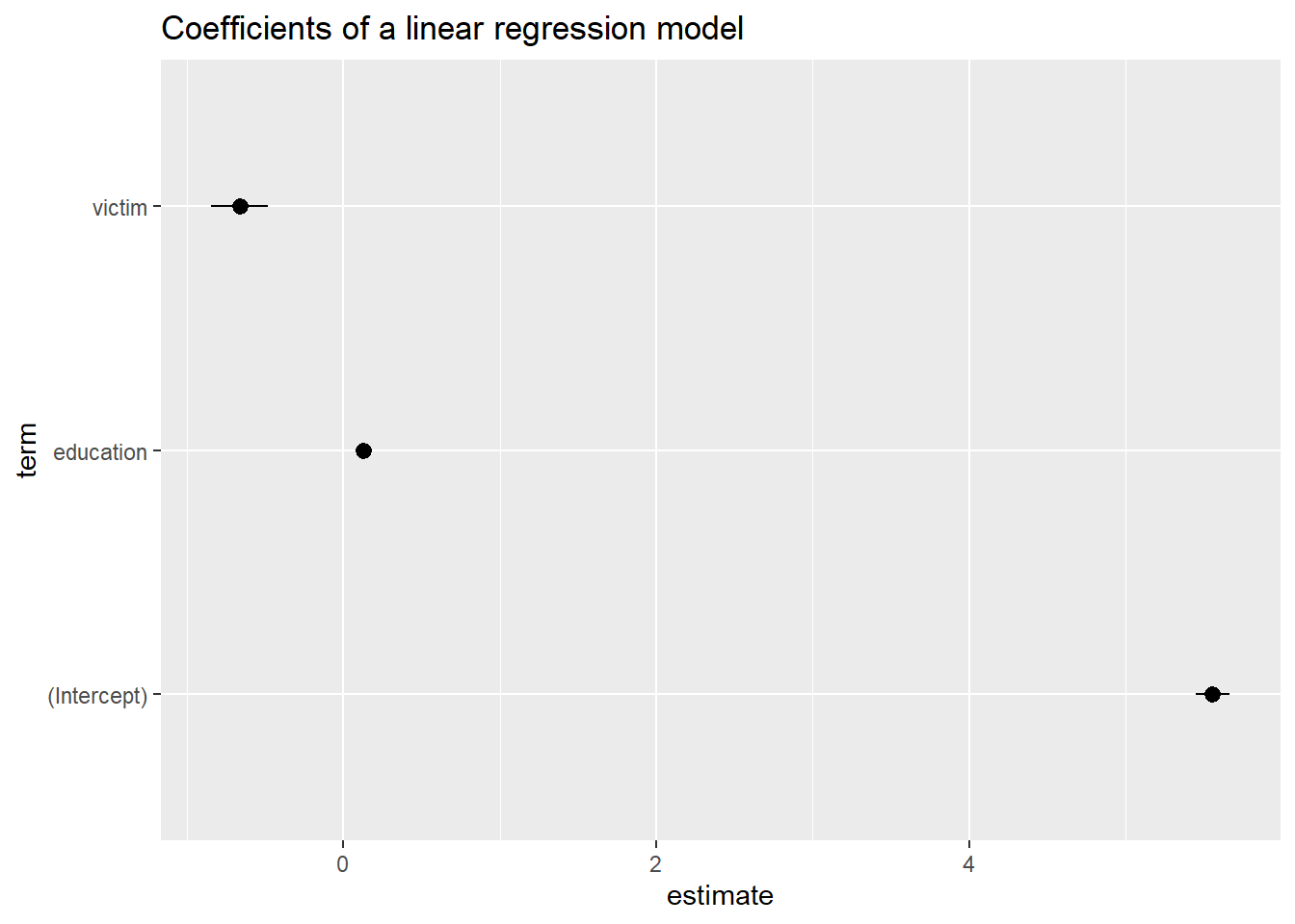
(Intercept)  5.558250   0.055462 100.217  < 2e-16 ***
victim      -0.662806   0.092424  -7.171 8.23e-13 ***
education    0.126997   0.009262  13.711  < 2e-16 ***
---
Signif. codes:  0 '***' 0.001 '**' 0.01 '*' 0.05 '.' 0.1 ' ' 1

Residual standard error: 2.261 on 6630 degrees of freedom
Multiple R-squared:  0.03631,   Adjusted R-squared:  0.03602 
F-statistic: 124.9 on 2 and 6630 DF,  p-value: < 2.2e-16
# Extract estimates
  tidy(M1, conf.int = TRUE) # conf.int ?
# A tibble: 3 x 7
  term        estimate std.error statistic  p.value conf.low conf.high
  <chr>          <dbl>     <dbl>     <dbl>    <dbl>    <dbl>     <dbl>
1 (Intercept)    5.56    0.0555     100.   0           5.45      5.67 
2 victim        -0.663   0.0924      -7.17 8.23e-13   -0.844    -0.482
3 education      0.127   0.00926     13.7  3.27e-42    0.109     0.145
  coefficients <- tidy(M1, conf.int = TRUE)

# Visualize estimates
  ggplot(coefficients, aes(term, estimate))+
    geom_point()+
    geom_pointrange(aes(ymin = conf.low, ymax = conf.high))+
    labs(title = "Coefficients of a linear regression model") +
    coord_flip()

# How can we exclude the intercept?
  # coefficients %>% ...


# Extract model statistics
  glance(M1)
# A tibble: 1 x 12
  r.squared adj.r.s~1 sigma stati~2  p.value    df  logLik    AIC    BIC devia~3
      <dbl>     <dbl> <dbl>   <dbl>    <dbl> <dbl>   <dbl>  <dbl>  <dbl>   <dbl>
1    0.0363    0.0360  2.26    125. 5.58e-54     2 -14822. 29651. 29678.  33893.
# ... with 2 more variables: df.residual <int>, nobs <int>, and abbreviated
#   variable names 1: adj.r.squared, 2: statistic, 3: deviance
  glance(M1)$r.squared
[1] 0.03631362
  glance(M1)$adj.r.squared
[1] 0.03602292
# Add predictions to data
  augment(M1) # Takes original data and appends predictions 
# A tibble: 6,633 x 9
   trust victim education .fitted  .resid     .hat .sigma      .cooksd .std.re~1
   <dbl>  <dbl>     <dbl>   <dbl>   <dbl>    <dbl>  <dbl>        <dbl>     <dbl>
 1     4      0         8    6.57 -2.57   0.000310   2.26 0.000134      -1.14   
 2     5      1         1    5.02 -0.0224 0.00172    2.26 0.0000000565  -0.00993
 3     0      0         0    5.56 -5.56   0.000602   2.26 0.00121       -2.46   
 4     5      0         9    6.70 -1.70   0.000425   2.26 0.0000802     -0.753  
 5     7      0         4    6.07  0.934  0.000187   2.26 0.0000107      0.413  
 6     5      0         1    5.69 -0.685  0.000448   2.26 0.0000137     -0.303  
 7     2      0         4    6.07 -4.07   0.000187   2.26 0.000202      -1.80   
 8     7      0         5    6.19  0.807  0.000168   2.26 0.00000712     0.357  
 9     7      0        10    6.83  0.172  0.000573   2.26 0.00000110     0.0760 
10     3      0         7    6.45 -3.45   0.000229   2.26 0.000178      -1.52   
# ... with 6,623 more rows, and abbreviated variable name 1: .std.resid
  # + errors + other things in the columns
  # What are the single columns? see ?augment -> value

1.2 Homework

  • Pick a dataset of your choice, estimate a linear model with an outcome of your choice. Extract the model coefficients using the tidy() function from the broom package, extract model statistics using the glance() function and add predicted values to the dataset using the augment() function.

1.3 All the code

library(tidyverse)
library(lemon)
library(knitr)

# install.packages("broom")
# install.packages("ggplot2")
library(broom)
library(ggplot2)

# Load data
  data <- read_csv(sprintf("https://docs.google.com/uc?id=%s&export=download",
                           "1I0eVUFyw0yn9T5roxzr67hPEl_5ZClrL"))

# Inspect the data
  data
  str(data)
  summary(data)
  # View(data)

# Estimate a linear model
  M1 <- lm(trust ~ victim + education,
           data = data)

# Check the output
  summary(M1)


# Extract estimates
  tidy(M1, conf.int = TRUE) # conf.int ?
  coefficients <- tidy(M1, conf.int = TRUE)

# Visualize estimates
  ggplot(coefficients, aes(term, estimate))+
    geom_point()+
    geom_pointrange(aes(ymin = conf.low, ymax = conf.high))+
    labs(title = "Coefficients of a linear regression model") +
    coord_flip()

# How can we exclude the intercept?
  # coefficients %>% ...


# Extract model statistics
  glance(M1)
  glance(M1)$r.squared
  glance(M1)$adj.r.squared
  
# Add predictions to data
  augment(M1) # Takes original data and appends predictions 
  # + errors + other things in the columns
  # What are the single columns? see ?augment -> value