Lab: Fairness and bias in predicting recidivism

Learning outcomes/objective: Learn…

• …how to assess whether an algorithm is biased.

Sources: Lee, Du, and Guerzhoy (2020)

1 Classifier performance & fairness (1): False positives & negatives

• Above: Correct Classification Rate (CCR) [as opposed to Error Rate]
  • For what proportion of the units does the correct output \(y_{i}\) match the classifier (predicted) output \(\hat{y}_{i}\)?
  • Proportion of reoffenders correctly predicted
  • See here and ?@fig-precision
    • \((TN + TP)/(TN + TP + FN + FP)\)
• False Positive Rate (FPR)
  • For what proportion of the units for which the correct output \(y_{i}\) is negative (=0, N in ?@fig-precision) is the classifier output \(\hat{y}_{i}\) positive (=1, FP in ?@fig-precision)?
  • Proportion of true NON reoffenders (NON recidivators) predicted as reoffenders (recidivators)
  • \(FP/N\)
• What then is the False Negative Rate (FNR) be?

2 Classifier performance & fairness (2)

• Algorithmic fairness can be assessed with respect to an input characteristic \(C\) (e.g., race, sex)
• False positive parity…
  • …is satisfied with respect to characteristic \(C\) if the false positive rate (\(FPR=FP/N\)) for inputs with \(C = 0\) (e.g., black) is the same as the false positive rate for inputs with \(C = 1\) (e.g., white)
  • ProPublica found that the false positive rate for African-American defendants (i.e., the percentage of innocent African-American defendants classified as likely to re-offend) was higher than for white defendants (NO false positive parity)
• Calibration…
  • …is satisfied with respect to characteristic \(C\) if an individual who was labeled “positive” has the same probability of actually being positive, regardless of the value of \(C\)…
  • …and if an individual who was labeled “negative” has the same probability of actually being negative regardless of the value of \(C\)
  • COMPAS makers claim that COMPAS satisfies calibration!

3 Lab: Classifier performance & fairness

See previous lab for notes.

# install.packages(pacman)
pacman::p_load(tidyverse,
               tidymodels,
               naniar,
               knitr,
               kableExtra)

We first import the data into R:

data <- read_csv(sprintf("https://docs.google.com/uc?id=%s&export=download",
                         "1plUxvMIoieEcCZXkBpj4Bxw1rDwa27tj"))

See previous lab for notes.

# Split the data into training and test data
  data_split <- initial_split(data, prop = 0.80)
  data_split # Inspect

<Training/Testing/Total>
<5771/1443/7214>

# Extract the two datasets
  data_train <- training(data_split)
  data_test <- testing(data_split) # Do not touch until the end!

# Further split the training data into analysis (training2) and assessment (validation) dataset 
  data_folds <- validation_split(data_train, prop = .80)
  data_folds # Inspect: We have only 1 fold!

# Validation Set Split (0.8/0.2)  
# A tibble: 1 x 2
  splits              id        
  <list>              <chr>     
1 <split [4616/1155]> validation

# Extract analysis ("training data 2") and assessment (validation) data
  data_analysis <- analysis(data_folds$splits[[1]])
  dim(data_analysis)

[1] 4616   53

  data_assessment <- assessment(data_folds$splits[[1]])
  dim(assessment)

NULL

See previous lab for notes.

fit <- glm(is_recid ~ age + priors_count, 
           family = binomial, 
           data = data_analysis)
#fit$coefficients
summary(fit)

Call:
glm(formula = is_recid ~ age + priors_count, family = binomial, 
    data = data_analysis)

Deviance Residuals: 
    Min       1Q   Median       3Q      Max  
-2.8497  -1.0541  -0.5628   1.1043   2.6117  

Coefficients:
              Estimate Std. Error z value Pr(>|z|)    
(Intercept)   1.043825   0.103062   10.13   <2e-16 ***
age          -0.049666   0.003038  -16.35   <2e-16 ***
priors_count  0.173625   0.008853   19.61   <2e-16 ***
---
Signif. codes:  0 '***' 0.001 '**' 0.01 '*' 0.05 '.' 0.1 ' ' 1

(Dispersion parameter for binomial family taken to be 1)

    Null deviance: 6388.5  on 4615  degrees of freedom
Residual deviance: 5667.9  on 4613  degrees of freedom
AIC: 5673.9

Number of Fisher Scoring iterations: 4

3.1 COMPAS scores: Fairness evaluation

Here, we are computing the False Positive Rate (FPR), False Negative Rate (FNR) and the correct classification rate (CCR) for different populations based on the COMPASS SCORES.To do so we use the validation data data_assessment. First, we’ll define functions get_FPR, get_FNR and get_CCR to compute the false positive rate (FPR), the false negative rate (FNR) and the correct classification rate (CCR). Below we describe the arguments in those functions:

• data_set argument is used to define the dataset, i.e., we can calculate these rates in data_analysis, data_assessment or data_test.
• thr argument in the functions is used to define the threshold (usually \(0.5\))
• outcome argument will contain the outcome variable is_recid which is the actual outcome variable
• probability_predicted argument is used to define the predicted probability
  • We use the the COMPAS score decile_score (above 5 predicted to recidivate) and our own model predictedion prediction further below

# Function: False Positive Rate
get_FPR <- function(data_set, # Use assessment or test data here
                    outcome, # Specify outcome variable
                    probability_predicted, # Specify var containted pred. probs.
                    thr) { # Specify threshold
  return( # display results
    # Sum above threshold AND NOT recidivate
    sum((data_set %>% select(all_of(probability_predicted)) >= thr) &
      (data_set %>% select(all_of(outcome)) == 0))
    / # divided by
      # Sum NOT recividate
      sum(data_set %>% select(all_of(outcome)) == 0)
  )
}
# Share of people over the threshold that did not recidivate
# of all that did not recidivate (who got falsely predicted to
# recidivate)

# Q: Please explain the function below!

# Function: False Negative Rate
get_FNR <- function(data_set,
                    outcome,
                    probability_predicted,
                    thr) {
  return(
    sum((data_set %>% select(all_of(probability_predicted)) < thr) &
      (data_set %>% select(all_of(outcome)) == 1)) # ?
    /
      sum(data_set %>% select(all_of(outcome)) == 1)
  ) # ?
}

# Q: Explain the function below!
# Function: Correct Classification Rate
get_CCR <- function(data_set,
                    outcome,
                    probability_predicted,
                    thr) {
  return(
    mean((data_set %>% select(all_of(probability_predicted)) >= thr) # ?
    ==
      data_set %>% select(all_of(outcome)))
  ) # ?
}

Let’s check out what ethic groups we have (complete dataset):

kable(table(data$race),
      col.names = c("Race", "Frequency"))

Race	Frequency
African-American	3696
Asian	32
Caucasian	2454
Hispanic	637
Native American	18
Other	377

We start by creating a nested dataframe data_assessment_groups that contains dataframes of data_assessment for all observations and subsets thereof (ethnic groups).

data_assessment_all <- data_assessment %>%
  mutate(race = "All") %>% # replace grouping variable with constant
  nest(.by = "race")
data_assessment_groups_race <- data_assessment %>%
  nest(.by = "race")

data_assessment_groups <- bind_rows(
  data_assessment_all,
  data_assessment_groups_race
)
data_assessment_groups

# A tibble: 7 x 2
  race             data                 
  <chr>            <list>               
1 All              <tibble [1,155 x 52]>
2 African-American <tibble [584 x 52]>  
3 Hispanic         <tibble [104 x 52]>  
4 Caucasian        <tibble [404 x 52]>  
5 Other            <tibble [57 x 52]>   
6 Asian            <tibble [4 x 52]>    
7 Native American  <tibble [2 x 52]>    

Then we apply our functions to data_assessment_groups with thr = \(5\) because COMPAS score decile_score, our predicted probability, goes from 0-10 instead of 0-1.

data_assessment_groups %>%
  mutate(
    FPR = map_dbl(
      .x = data,
      ~ get_FPR(
        data_set = .x,
        outcome = "is_recid",
        probability_predicted = "decile_score",
        thr = 5
      )
    ),
    FNR = map_dbl(
      .x = data,
      ~ get_FNR(
        data_set = .x,
        outcome = "is_recid",
        probability_predicted = "decile_score",
        thr = 5
      )
    ),
    CCR = map_dbl(
      .x = data,
      ~ get_CCR(
        data_set = .x,
        outcome = "is_recid",
        probability_predicted = "decile_score",
        thr = 5
      )
    )
  ) %>%
  mutate_if(is.numeric, round, digits = 2)

# A tibble: 7 x 5
  race             data                    FPR   FNR   CCR
  <chr>            <list>                <dbl> <dbl> <dbl>
1 All              <tibble [1,155 x 52]>  0.32  0.39  0.65
2 African-American <tibble [584 x 52]>    0.45  0.28  0.64
3 Hispanic         <tibble [104 x 52]>    0.15  0.63  0.65
4 Caucasian        <tibble [404 x 52]>    0.26  0.5   0.64
5 Other            <tibble [57 x 52]>     0.14  0.62  0.68
6 Asian            <tibble [4 x 52]>      0     0     1   
7 Native American  <tibble [2 x 52]>      0     0     1   

We can see that the scores do not satisfy false positive parity and do not satisfy false negative parity. The scores do satisfy classification parity. Demographic parity is also not satisfied.

3.2 Our model: Fairness evaluation

Let’s now obtain the FPR, FNR, and CCR for our own predictive logistic regression model, using the threshold \(0.5\). In the functions below we first generate predicted values for our outcome is_recid using the predict() function. Then we basically do the same as above, however, now we don’t use the COMPAS scores stored in decile_score but use our own predicted values stored in the variable prediction. The predicted values are between 0 and 1 and not deciles as in decile_score. Hence, we have to change thr from \(5\) to \(0.5\).

# Add predictions to data
data_assessment <- data_assessment %>%
  mutate(prediction = predict(fit,
    newdata = .,
    type = "response"
  ))

data_assessment_all <- data_assessment %>%
  mutate(race = "All") %>% # replace grouping variable with constant
  nest(.by = "race")
data_assessment_groups_race <- data_assessment %>%
  nest(.by = "race")

data_assessment_groups <- bind_rows(
  data_assessment_all,
  data_assessment_groups_race
)


data_assessment_groups %>%
  mutate(
    FPR = map_dbl(
      .x = data,
      ~ get_FPR(
        data_set = .x,
        outcome = "is_recid",
        probability_predicted = "prediction",
        thr = 0.5
      )
    ),
    FNR = map_dbl(
      .x = data,
      ~ get_FNR(
        data_set = .x,
        outcome = "is_recid",
        probability_predicted = "prediction",
        thr = 0.5
      )
    ),
    CCR = map_dbl(
      .x = data,
      ~ get_CCR(
        data_set = .x,
        outcome = "is_recid",
        probability_predicted = "prediction",
        thr = 0.5
      )
    )
  ) %>%
  mutate_if(is.numeric, round, digits = 2)

# A tibble: 7 x 5
  race             data                    FPR   FNR   CCR
  <chr>            <list>                <dbl> <dbl> <dbl>
1 All              <tibble [1,155 x 53]>  0.26  0.4   0.67
2 African-American <tibble [584 x 53]>    0.35  0.28  0.69
3 Hispanic         <tibble [104 x 53]>    0.21  0.53  0.65
4 Caucasian        <tibble [404 x 53]>    0.17  0.59  0.65
5 Other            <tibble [57 x 53]>     0.25  0.52  0.65
6 Asian            <tibble [4 x 53]>      0     1     0.75
7 Native American  <tibble [2 x 53]>      0     0     1   

We can see that the FPR is higher for African-Americans as compared to Caucasians (the FNR is lower). Hence, they are treated unfairly.

3.3 Altering the threshold (of our model!)

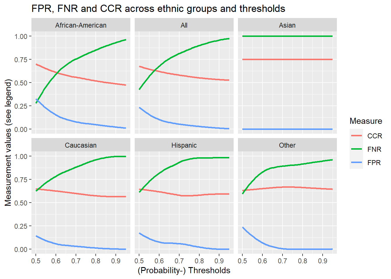
We can also explore how changing the threshold influences the false positive, false negative, and correct classification rates for the different ethnic groups. Below we use a combination of expand(), nesting() and map() with our functions to produce and visualize the corresponding data. You can execute the code step by step (from pipe to pipe).

# Define threshold values
thrs <- seq(0.5, 0.95, 0.01)

# Expand df with threshold values and calculate rates
data_assessment_groups %>%
  filter(race != "Native American") %>% # too few observations
  expand(nesting(race, data), thrs) %>%
  mutate(
    FPR = map2_dbl(
      .x = data,
      .y = thrs,
      ~ get_FPR(
        data_set = .x,
        outcome = "is_recid",
        probability_predicted = "prediction",
        thr = .y
      )
    ),
    FNR = map2_dbl(
      .x = data,
      .y = thrs,
      ~ get_FNR(
        data_set = .x,
        outcome = "is_recid",
        probability_predicted = "prediction",
        thr = .y
      )
    ),
    CCR = map2_dbl(
      .x = data,
      .y = thrs,
      ~ get_CCR(
        data_set = .x,
        outcome = "is_recid",
        probability_predicted = "prediction",
        thr = .y
      )
    )
  ) %>%
  pivot_longer(
    cols = FPR:CCR,
    names_to = "measure",
    values_to = "value"
  ) %>%
  ggplot(mapping = aes(
    x = thrs,
    y = value,
    color = measure
  )) +
  geom_smooth(
    se = F,
    method = "loess"
  ) +
  facet_wrap(~race) +
  labs(
    title = "FPR, FNR and CCR across ethnic groups and thresholds",
    x = "(Probability-) Thresholds",
    y = "Measurement values (see legend)",
    color = "Measure"
  )

3.4 Adjusting thresholds

In the end, we basically want to know how to we would need to adapt the thresholds for different groups (especially African-Americans) so that their false positive rates are at parity with Caucasians. In other words we would like to find the thresholds for which the false positive rates are at parity. Let’s see what the rates are for different thresholds. We reuse data_assessment_groups from above.

# Define threshold values
thrs <- seq(0.5, 0.95, 0.0005)

comparison_thresholds <- data_assessment_groups %>%
  filter(race == "African-American" | race == "Caucasian") %>% # too few observations
  expand(nesting(race, data), thrs) %>%
  mutate(FPR = map2_dbl(
    .x = data,
    .y = thrs,
    ~ get_FPR(
      data_set = .x,
      outcome = "is_recid",
      probability_predicted = "prediction",
      thr = .y
    )
  )) %>%
  select(-data) %>%
  pivot_wider(
    names_from = "race",
    values_from = "FPR",
    names_prefix = "FPR_"
  )

comparison_thresholds %>%
  kable() %>%
  kable_styling("striped", full_width = T) %>%
  scroll_box(height = "200px")

thrs	FPR_African-American	FPR_Caucasian
0.5000	0.3544776	0.1666667
0.5005	0.3320896	0.1403509
0.5010	0.3320896	0.1403509
0.5015	0.3320896	0.1403509
0.5020	0.3320896	0.1403509
0.5025	0.3320896	0.1403509
0.5030	0.3320896	0.1403509
0.5035	0.3320896	0.1403509
0.5040	0.3320896	0.1403509
0.5045	0.3320896	0.1403509
0.5050	0.3320896	0.1403509
0.5055	0.3320896	0.1403509
0.5060	0.3320896	0.1403509
0.5065	0.3208955	0.1359649
0.5070	0.3208955	0.1359649
0.5075	0.3208955	0.1359649
0.5080	0.3208955	0.1359649
0.5085	0.3208955	0.1359649
0.5090	0.3208955	0.1359649
0.5095	0.3208955	0.1359649
0.5100	0.3208955	0.1359649
0.5105	0.3208955	0.1359649
0.5110	0.3208955	0.1359649
0.5115	0.3208955	0.1359649
0.5120	0.3208955	0.1359649
0.5125	0.3208955	0.1359649
0.5130	0.2910448	0.1315789
0.5135	0.2910448	0.1315789
0.5140	0.2910448	0.1315789
0.5145	0.2910448	0.1315789
0.5150	0.2910448	0.1315789
0.5155	0.2910448	0.1315789
0.5160	0.2910448	0.1315789
0.5165	0.2910448	0.1315789
0.5170	0.2910448	0.1315789
0.5175	0.2910448	0.1315789
0.5180	0.2910448	0.1315789
0.5185	0.2910448	0.1315789
0.5190	0.2649254	0.1184211
0.5195	0.2649254	0.1184211
0.5200	0.2649254	0.1184211
0.5205	0.2649254	0.1184211
0.5210	0.2649254	0.1184211
0.5215	0.2649254	0.1184211
0.5220	0.2649254	0.1184211
0.5225	0.2649254	0.1184211
0.5230	0.2649254	0.1184211
0.5235	0.2649254	0.1184211
0.5240	0.2649254	0.1184211
0.5245	0.2611940	0.1184211
0.5250	0.2537313	0.1096491
0.5255	0.2537313	0.1096491
0.5260	0.2537313	0.1096491
0.5265	0.2537313	0.1096491
0.5270	0.2537313	0.1096491
0.5275	0.2537313	0.1096491
0.5280	0.2537313	0.1096491
0.5285	0.2537313	0.1096491
0.5290	0.2537313	0.1096491
0.5295	0.2537313	0.1096491
0.5300	0.2537313	0.1096491
0.5305	0.2537313	0.1096491
0.5310	0.2500000	0.1096491
0.5315	0.2462687	0.1008772
0.5320	0.2462687	0.1008772
0.5325	0.2462687	0.1008772
0.5330	0.2462687	0.1008772
0.5335	0.2462687	0.1008772
0.5340	0.2462687	0.1008772
0.5345	0.2462687	0.1008772
0.5350	0.2462687	0.1008772
0.5355	0.2462687	0.1008772
0.5360	0.2462687	0.1008772
0.5365	0.2462687	0.1008772
0.5370	0.2462687	0.1008772
0.5375	0.2425373	0.0964912
0.5380	0.2425373	0.0964912
0.5385	0.2425373	0.0964912
0.5390	0.2425373	0.0964912
0.5395	0.2425373	0.0964912
0.5400	0.2425373	0.0964912
0.5405	0.2425373	0.0964912
0.5410	0.2425373	0.0964912
0.5415	0.2425373	0.0964912
0.5420	0.2425373	0.0964912
0.5425	0.2425373	0.0964912
0.5430	0.2425373	0.0964912
0.5435	0.2388060	0.0877193
0.5440	0.2126866	0.0789474
0.5445	0.2126866	0.0789474
0.5450	0.2126866	0.0789474
0.5455	0.2126866	0.0789474
0.5460	0.2126866	0.0789474
0.5465	0.2126866	0.0789474
0.5470	0.2126866	0.0789474
0.5475	0.2126866	0.0789474
0.5480	0.2126866	0.0789474
0.5485	0.2126866	0.0789474
0.5490	0.2126866	0.0789474
0.5495	0.2126866	0.0789474
0.5500	0.2089552	0.0789474
0.5505	0.2089552	0.0789474
0.5510	0.2089552	0.0789474
0.5515	0.2089552	0.0789474
0.5520	0.2089552	0.0789474
0.5525	0.2089552	0.0789474
0.5530	0.2089552	0.0789474
0.5535	0.2089552	0.0789474
0.5540	0.2089552	0.0789474
0.5545	0.2089552	0.0789474
0.5550	0.2089552	0.0789474
0.5555	0.2052239	0.0789474
0.5560	0.2014925	0.0745614
0.5565	0.2014925	0.0745614
0.5570	0.2014925	0.0745614
0.5575	0.2014925	0.0745614
0.5580	0.2014925	0.0745614
0.5585	0.2014925	0.0745614
0.5590	0.2014925	0.0745614
0.5595	0.2014925	0.0745614
0.5600	0.2014925	0.0745614
0.5605	0.2014925	0.0745614
0.5610	0.2014925	0.0745614
0.5615	0.2014925	0.0745614
0.5620	0.1865672	0.0657895
0.5625	0.1865672	0.0657895
0.5630	0.1865672	0.0657895
0.5635	0.1865672	0.0657895
0.5640	0.1865672	0.0657895
0.5645	0.1865672	0.0657895
0.5650	0.1865672	0.0657895
0.5655	0.1865672	0.0657895
0.5660	0.1865672	0.0657895
0.5665	0.1865672	0.0657895
0.5670	0.1865672	0.0657895
0.5675	0.1865672	0.0657895
0.5680	0.1828358	0.0614035
0.5685	0.1828358	0.0614035
0.5690	0.1828358	0.0614035
0.5695	0.1828358	0.0614035
0.5700	0.1828358	0.0614035
0.5705	0.1828358	0.0614035
0.5710	0.1828358	0.0614035
0.5715	0.1828358	0.0614035
0.5720	0.1828358	0.0614035
0.5725	0.1828358	0.0614035
0.5730	0.1828358	0.0614035
0.5735	0.1828358	0.0614035
0.5740	0.1679104	0.0570175
0.5745	0.1641791	0.0570175
0.5750	0.1641791	0.0570175
0.5755	0.1641791	0.0570175
0.5760	0.1641791	0.0570175
0.5765	0.1641791	0.0570175
0.5770	0.1641791	0.0570175
0.5775	0.1641791	0.0570175
0.5780	0.1641791	0.0570175
0.5785	0.1641791	0.0570175
0.5790	0.1641791	0.0570175
0.5795	0.1641791	0.0570175
0.5800	0.1604478	0.0570175
0.5805	0.1567164	0.0570175
0.5810	0.1567164	0.0570175
0.5815	0.1567164	0.0570175
0.5820	0.1567164	0.0570175
0.5825	0.1567164	0.0570175
0.5830	0.1567164	0.0570175
0.5835	0.1567164	0.0570175
0.5840	0.1567164	0.0570175
0.5845	0.1567164	0.0570175
0.5850	0.1567164	0.0570175
0.5855	0.1567164	0.0570175
0.5860	0.1567164	0.0570175
0.5865	0.1492537	0.0526316
0.5870	0.1492537	0.0526316
0.5875	0.1492537	0.0526316
0.5880	0.1492537	0.0526316
0.5885	0.1492537	0.0526316
0.5890	0.1492537	0.0526316
0.5895	0.1492537	0.0526316
0.5900	0.1492537	0.0526316
0.5905	0.1492537	0.0526316
0.5910	0.1492537	0.0526316
0.5915	0.1492537	0.0526316
0.5920	0.1492537	0.0526316
0.5925	0.1492537	0.0526316
0.5930	0.1492537	0.0526316
0.5935	0.1492537	0.0526316
0.5940	0.1492537	0.0526316
0.5945	0.1492537	0.0526316
0.5950	0.1492537	0.0526316
0.5955	0.1492537	0.0526316
0.5960	0.1492537	0.0526316
0.5965	0.1492537	0.0526316
0.5970	0.1492537	0.0526316
0.5975	0.1492537	0.0526316
0.5980	0.1417910	0.0526316
0.5985	0.1417910	0.0526316
0.5990	0.1417910	0.0526316
0.5995	0.1417910	0.0526316
0.6000	0.1417910	0.0526316
0.6005	0.1417910	0.0526316
0.6010	0.1417910	0.0526316
0.6015	0.1417910	0.0526316
0.6020	0.1417910	0.0526316
0.6025	0.1417910	0.0526316
0.6030	0.1417910	0.0526316
0.6035	0.1417910	0.0526316
0.6040	0.1380597	0.0526316
0.6045	0.1380597	0.0526316
0.6050	0.1380597	0.0526316
0.6055	0.1380597	0.0526316
0.6060	0.1380597	0.0526316
0.6065	0.1380597	0.0526316
0.6070	0.1380597	0.0526316
0.6075	0.1380597	0.0526316
0.6080	0.1380597	0.0526316
0.6085	0.1380597	0.0526316
0.6090	0.1380597	0.0526316
0.6095	0.1380597	0.0526316
0.6100	0.1380597	0.0526316
0.6105	0.1380597	0.0526316
0.6110	0.1380597	0.0526316
0.6115	0.1380597	0.0526316
0.6120	0.1380597	0.0526316
0.6125	0.1380597	0.0526316
0.6130	0.1380597	0.0526316
0.6135	0.1380597	0.0526316
0.6140	0.1380597	0.0526316
0.6145	0.1380597	0.0526316
0.6150	0.1380597	0.0526316
0.6155	0.1380597	0.0526316
0.6160	0.1343284	0.0526316
0.6165	0.1343284	0.0526316
0.6170	0.1343284	0.0526316
0.6175	0.1343284	0.0526316
0.6180	0.1343284	0.0526316
0.6185	0.1343284	0.0526316
0.6190	0.1343284	0.0526316
0.6195	0.1343284	0.0526316
0.6200	0.1343284	0.0526316
0.6205	0.1343284	0.0526316
0.6210	0.1343284	0.0526316
0.6215	0.1343284	0.0482456
0.6220	0.1343284	0.0438596
0.6225	0.1343284	0.0438596
0.6230	0.1343284	0.0438596
0.6235	0.1343284	0.0438596
0.6240	0.1343284	0.0438596
0.6245	0.1343284	0.0438596
0.6250	0.1343284	0.0438596
0.6255	0.1343284	0.0438596
0.6260	0.1343284	0.0438596
0.6265	0.1343284	0.0438596
0.6270	0.1343284	0.0438596
0.6275	0.1268657	0.0438596
0.6280	0.1268657	0.0438596
0.6285	0.1268657	0.0438596
0.6290	0.1268657	0.0438596
0.6295	0.1268657	0.0438596
0.6300	0.1268657	0.0438596
0.6305	0.1268657	0.0438596
0.6310	0.1268657	0.0438596
0.6315	0.1268657	0.0438596
0.6320	0.1268657	0.0438596
0.6325	0.1268657	0.0438596
0.6330	0.1268657	0.0438596
0.6335	0.1268657	0.0394737
0.6340	0.1268657	0.0394737
0.6345	0.1268657	0.0394737
0.6350	0.1268657	0.0394737
0.6355	0.1268657	0.0394737
0.6360	0.1268657	0.0394737
0.6365	0.1268657	0.0394737
0.6370	0.1268657	0.0394737
0.6375	0.1268657	0.0394737
0.6380	0.1268657	0.0394737
0.6385	0.1268657	0.0394737
0.6390	0.1194030	0.0394737
0.6395	0.1194030	0.0394737
0.6400	0.1194030	0.0394737
0.6405	0.1194030	0.0394737
0.6410	0.1194030	0.0394737
0.6415	0.1194030	0.0394737
0.6420	0.1194030	0.0394737
0.6425	0.1194030	0.0394737
0.6430	0.1194030	0.0394737
0.6435	0.1194030	0.0394737
0.6440	0.1194030	0.0394737
0.6445	0.1194030	0.0394737
0.6450	0.1119403	0.0394737
0.6455	0.1119403	0.0394737
0.6460	0.1119403	0.0394737
0.6465	0.1119403	0.0394737
0.6470	0.1119403	0.0394737
0.6475	0.1119403	0.0394737
0.6480	0.1119403	0.0394737
0.6485	0.1119403	0.0394737
0.6490	0.1119403	0.0394737
0.6495	0.1119403	0.0394737
0.6500	0.1119403	0.0394737
0.6505	0.1044776	0.0394737
0.6510	0.1044776	0.0394737
0.6515	0.1044776	0.0394737
0.6520	0.1044776	0.0394737
0.6525	0.1044776	0.0394737
0.6530	0.1044776	0.0394737
0.6535	0.1044776	0.0394737
0.6540	0.1044776	0.0394737
0.6545	0.1044776	0.0394737
0.6550	0.1044776	0.0394737
0.6555	0.1044776	0.0394737
0.6560	0.1044776	0.0394737
0.6565	0.1044776	0.0394737
0.6570	0.1044776	0.0394737
0.6575	0.1044776	0.0394737
0.6580	0.1044776	0.0394737
0.6585	0.1044776	0.0394737
0.6590	0.1044776	0.0394737
0.6595	0.1044776	0.0394737
0.6600	0.1044776	0.0394737
0.6605	0.1044776	0.0394737
0.6610	0.1044776	0.0394737
0.6615	0.1007463	0.0394737
0.6620	0.0932836	0.0394737
0.6625	0.0932836	0.0394737
0.6630	0.0932836	0.0394737
0.6635	0.0932836	0.0394737
0.6640	0.0932836	0.0394737
0.6645	0.0932836	0.0394737
0.6650	0.0932836	0.0394737
0.6655	0.0932836	0.0394737
0.6660	0.0932836	0.0394737
0.6665	0.0932836	0.0394737
0.6670	0.0932836	0.0394737
0.6675	0.0895522	0.0394737
0.6680	0.0895522	0.0394737
0.6685	0.0895522	0.0394737
0.6690	0.0895522	0.0394737
0.6695	0.0895522	0.0394737
0.6700	0.0895522	0.0394737
0.6705	0.0895522	0.0394737
0.6710	0.0895522	0.0394737
0.6715	0.0895522	0.0394737
0.6720	0.0895522	0.0394737
0.6725	0.0895522	0.0394737
0.6730	0.0895522	0.0394737
0.6735	0.0895522	0.0394737
0.6740	0.0895522	0.0394737
0.6745	0.0895522	0.0394737
0.6750	0.0895522	0.0394737
0.6755	0.0895522	0.0394737
0.6760	0.0895522	0.0394737
0.6765	0.0895522	0.0394737
0.6770	0.0895522	0.0394737
0.6775	0.0895522	0.0394737
0.6780	0.0895522	0.0350877
0.6785	0.0895522	0.0350877
0.6790	0.0895522	0.0350877
0.6795	0.0895522	0.0350877
0.6800	0.0895522	0.0350877
0.6805	0.0895522	0.0350877
0.6810	0.0895522	0.0350877
0.6815	0.0895522	0.0350877
0.6820	0.0895522	0.0350877
0.6825	0.0895522	0.0350877
0.6830	0.0895522	0.0350877
0.6835	0.0895522	0.0350877
0.6840	0.0895522	0.0350877
0.6845	0.0895522	0.0350877
0.6850	0.0895522	0.0350877
0.6855	0.0895522	0.0350877
0.6860	0.0895522	0.0350877
0.6865	0.0895522	0.0350877
0.6870	0.0895522	0.0350877
0.6875	0.0895522	0.0350877
0.6880	0.0895522	0.0350877
0.6885	0.0895522	0.0350877
0.6890	0.0858209	0.0350877
0.6895	0.0858209	0.0350877
0.6900	0.0858209	0.0350877
0.6905	0.0858209	0.0350877
0.6910	0.0858209	0.0350877
0.6915	0.0858209	0.0350877
0.6920	0.0858209	0.0350877
0.6925	0.0858209	0.0350877
0.6930	0.0858209	0.0350877
0.6935	0.0858209	0.0350877
0.6940	0.0858209	0.0307018
0.6945	0.0858209	0.0307018
0.6950	0.0858209	0.0307018
0.6955	0.0858209	0.0307018
0.6960	0.0858209	0.0307018
0.6965	0.0858209	0.0307018
0.6970	0.0858209	0.0307018
0.6975	0.0858209	0.0307018
0.6980	0.0858209	0.0307018
0.6985	0.0858209	0.0307018
0.6990	0.0858209	0.0307018
0.6995	0.0783582	0.0307018
0.7000	0.0783582	0.0307018
0.7005	0.0783582	0.0307018
0.7010	0.0783582	0.0307018
0.7015	0.0783582	0.0307018
0.7020	0.0783582	0.0307018
0.7025	0.0783582	0.0307018
0.7030	0.0783582	0.0307018
0.7035	0.0783582	0.0307018
0.7040	0.0783582	0.0307018
0.7045	0.0708955	0.0307018
0.7050	0.0708955	0.0307018
0.7055	0.0708955	0.0307018
0.7060	0.0708955	0.0307018
0.7065	0.0708955	0.0307018
0.7070	0.0708955	0.0307018
0.7075	0.0708955	0.0307018
0.7080	0.0708955	0.0307018
0.7085	0.0708955	0.0307018
0.7090	0.0708955	0.0307018
0.7095	0.0708955	0.0307018
0.7100	0.0671642	0.0307018
0.7105	0.0671642	0.0307018
0.7110	0.0671642	0.0307018
0.7115	0.0671642	0.0307018
0.7120	0.0671642	0.0307018
0.7125	0.0671642	0.0307018
0.7130	0.0671642	0.0307018
0.7135	0.0671642	0.0307018
0.7140	0.0671642	0.0307018
0.7145	0.0671642	0.0307018
0.7150	0.0634328	0.0307018
0.7155	0.0634328	0.0307018
0.7160	0.0634328	0.0307018
0.7165	0.0634328	0.0307018
0.7170	0.0634328	0.0307018
0.7175	0.0634328	0.0307018
0.7180	0.0634328	0.0307018
0.7185	0.0634328	0.0307018
0.7190	0.0634328	0.0307018
0.7195	0.0634328	0.0307018
0.7200	0.0634328	0.0307018
0.7205	0.0634328	0.0307018
0.7210	0.0634328	0.0307018
0.7215	0.0634328	0.0307018
0.7220	0.0634328	0.0307018
0.7225	0.0634328	0.0307018
0.7230	0.0634328	0.0307018
0.7235	0.0634328	0.0307018
0.7240	0.0634328	0.0307018
0.7245	0.0634328	0.0307018
0.7250	0.0634328	0.0307018
0.7255	0.0634328	0.0307018
0.7260	0.0634328	0.0307018
0.7265	0.0634328	0.0307018
0.7270	0.0634328	0.0307018
0.7275	0.0634328	0.0307018
0.7280	0.0634328	0.0307018
0.7285	0.0634328	0.0307018
0.7290	0.0634328	0.0307018
0.7295	0.0634328	0.0263158
0.7300	0.0597015	0.0263158
0.7305	0.0597015	0.0263158
0.7310	0.0597015	0.0263158
0.7315	0.0597015	0.0263158
0.7320	0.0597015	0.0263158
0.7325	0.0597015	0.0263158
0.7330	0.0597015	0.0263158
0.7335	0.0597015	0.0263158
0.7340	0.0597015	0.0263158
0.7345	0.0559701	0.0263158
0.7350	0.0559701	0.0263158
0.7355	0.0559701	0.0263158
0.7360	0.0559701	0.0263158
0.7365	0.0559701	0.0263158
0.7370	0.0559701	0.0263158
0.7375	0.0559701	0.0263158
0.7380	0.0559701	0.0263158
0.7385	0.0559701	0.0263158
0.7390	0.0559701	0.0263158
0.7395	0.0559701	0.0263158
0.7400	0.0559701	0.0263158
0.7405	0.0559701	0.0263158
0.7410	0.0559701	0.0263158
0.7415	0.0559701	0.0263158
0.7420	0.0559701	0.0263158
0.7425	0.0559701	0.0263158
0.7430	0.0559701	0.0263158
0.7435	0.0559701	0.0263158
0.7440	0.0559701	0.0263158
0.7445	0.0559701	0.0219298
0.7450	0.0559701	0.0219298
0.7455	0.0559701	0.0219298
0.7460	0.0559701	0.0219298
0.7465	0.0559701	0.0219298
0.7470	0.0559701	0.0219298
0.7475	0.0559701	0.0219298
0.7480	0.0559701	0.0219298
0.7485	0.0559701	0.0219298
0.7490	0.0559701	0.0175439
0.7495	0.0559701	0.0175439
0.7500	0.0559701	0.0175439
0.7505	0.0559701	0.0175439
0.7510	0.0559701	0.0175439
0.7515	0.0559701	0.0175439
0.7520	0.0559701	0.0175439
0.7525	0.0559701	0.0175439
0.7530	0.0559701	0.0175439
0.7535	0.0559701	0.0175439
0.7540	0.0559701	0.0175439
0.7545	0.0559701	0.0175439
0.7550	0.0559701	0.0175439
0.7555	0.0559701	0.0175439
0.7560	0.0559701	0.0175439
0.7565	0.0559701	0.0175439
0.7570	0.0559701	0.0175439
0.7575	0.0559701	0.0175439
0.7580	0.0559701	0.0131579
0.7585	0.0559701	0.0131579
0.7590	0.0559701	0.0131579
0.7595	0.0559701	0.0131579
0.7600	0.0559701	0.0131579
0.7605	0.0559701	0.0131579
0.7610	0.0559701	0.0131579
0.7615	0.0559701	0.0131579
0.7620	0.0559701	0.0131579
0.7625	0.0559701	0.0131579
0.7630	0.0559701	0.0131579
0.7635	0.0559701	0.0131579
0.7640	0.0559701	0.0131579
0.7645	0.0559701	0.0131579
0.7650	0.0559701	0.0131579
0.7655	0.0559701	0.0131579
0.7660	0.0559701	0.0131579
0.7665	0.0559701	0.0131579
0.7670	0.0559701	0.0131579
0.7675	0.0559701	0.0131579
0.7680	0.0559701	0.0131579
0.7685	0.0559701	0.0131579
0.7690	0.0559701	0.0131579
0.7695	0.0559701	0.0131579
0.7700	0.0559701	0.0131579
0.7705	0.0559701	0.0131579
0.7710	0.0559701	0.0131579
0.7715	0.0559701	0.0131579
0.7720	0.0559701	0.0131579
0.7725	0.0559701	0.0131579
0.7730	0.0559701	0.0131579
0.7735	0.0559701	0.0131579
0.7740	0.0559701	0.0131579
0.7745	0.0559701	0.0131579
0.7750	0.0559701	0.0131579
0.7755	0.0559701	0.0131579
0.7760	0.0559701	0.0131579
0.7765	0.0559701	0.0131579
0.7770	0.0559701	0.0131579
0.7775	0.0559701	0.0131579
0.7780	0.0559701	0.0131579
0.7785	0.0559701	0.0131579
0.7790	0.0559701	0.0131579
0.7795	0.0559701	0.0131579
0.7800	0.0559701	0.0131579
0.7805	0.0559701	0.0131579
0.7810	0.0559701	0.0131579
0.7815	0.0559701	0.0131579
0.7820	0.0559701	0.0131579
0.7825	0.0559701	0.0131579
0.7830	0.0559701	0.0131579
0.7835	0.0559701	0.0131579
0.7840	0.0559701	0.0131579
0.7845	0.0559701	0.0131579
0.7850	0.0559701	0.0131579
0.7855	0.0559701	0.0131579
0.7860	0.0559701	0.0131579
0.7865	0.0559701	0.0131579
0.7870	0.0559701	0.0131579
0.7875	0.0559701	0.0131579
0.7880	0.0559701	0.0131579
0.7885	0.0559701	0.0131579
0.7890	0.0559701	0.0131579
0.7895	0.0559701	0.0131579
0.7900	0.0559701	0.0131579
0.7905	0.0559701	0.0131579
0.7910	0.0559701	0.0131579
0.7915	0.0559701	0.0131579
0.7920	0.0559701	0.0131579
0.7925	0.0559701	0.0131579
0.7930	0.0559701	0.0131579
0.7935	0.0559701	0.0131579
0.7940	0.0559701	0.0131579
0.7945	0.0559701	0.0131579
0.7950	0.0559701	0.0131579
0.7955	0.0559701	0.0131579
0.7960	0.0559701	0.0131579
0.7965	0.0559701	0.0131579
0.7970	0.0559701	0.0131579
0.7975	0.0559701	0.0131579
0.7980	0.0559701	0.0131579
0.7985	0.0559701	0.0131579
0.7990	0.0559701	0.0131579
0.7995	0.0559701	0.0131579
0.8000	0.0559701	0.0131579
0.8005	0.0559701	0.0131579
0.8010	0.0559701	0.0131579
0.8015	0.0559701	0.0131579
0.8020	0.0559701	0.0131579
0.8025	0.0559701	0.0131579
0.8030	0.0559701	0.0131579
0.8035	0.0559701	0.0131579
0.8040	0.0559701	0.0131579
0.8045	0.0559701	0.0131579
0.8050	0.0559701	0.0131579
0.8055	0.0559701	0.0131579
0.8060	0.0559701	0.0131579
0.8065	0.0559701	0.0131579
0.8070	0.0559701	0.0131579
0.8075	0.0559701	0.0131579
0.8080	0.0559701	0.0131579
0.8085	0.0485075	0.0131579
0.8090	0.0485075	0.0131579
0.8095	0.0485075	0.0131579
0.8100	0.0485075	0.0131579
0.8105	0.0485075	0.0131579
0.8110	0.0485075	0.0131579
0.8115	0.0485075	0.0131579
0.8120	0.0485075	0.0131579
0.8125	0.0447761	0.0087719
0.8130	0.0447761	0.0087719
0.8135	0.0447761	0.0087719
0.8140	0.0447761	0.0087719
0.8145	0.0447761	0.0087719
0.8150	0.0447761	0.0087719
0.8155	0.0447761	0.0087719
0.8160	0.0447761	0.0087719
0.8165	0.0447761	0.0087719
0.8170	0.0447761	0.0087719
0.8175	0.0447761	0.0087719
0.8180	0.0447761	0.0087719
0.8185	0.0447761	0.0087719
0.8190	0.0447761	0.0087719
0.8195	0.0447761	0.0087719
0.8200	0.0447761	0.0087719
0.8205	0.0447761	0.0087719
0.8210	0.0447761	0.0087719
0.8215	0.0447761	0.0087719
0.8220	0.0447761	0.0087719
0.8225	0.0447761	0.0087719
0.8230	0.0447761	0.0087719
0.8235	0.0447761	0.0087719
0.8240	0.0447761	0.0087719
0.8245	0.0447761	0.0087719
0.8250	0.0447761	0.0087719
0.8255	0.0447761	0.0087719
0.8260	0.0447761	0.0087719
0.8265	0.0447761	0.0087719
0.8270	0.0447761	0.0087719
0.8275	0.0447761	0.0087719
0.8280	0.0447761	0.0087719
0.8285	0.0447761	0.0087719
0.8290	0.0447761	0.0087719
0.8295	0.0447761	0.0087719
0.8300	0.0447761	0.0087719
0.8305	0.0373134	0.0087719
0.8310	0.0373134	0.0087719
0.8315	0.0373134	0.0087719
0.8320	0.0373134	0.0087719
0.8325	0.0373134	0.0087719
0.8330	0.0373134	0.0087719
0.8335	0.0373134	0.0087719
0.8340	0.0373134	0.0087719
0.8345	0.0373134	0.0087719
0.8350	0.0373134	0.0087719
0.8355	0.0373134	0.0087719
0.8360	0.0373134	0.0087719
0.8365	0.0373134	0.0087719
0.8370	0.0373134	0.0087719
0.8375	0.0373134	0.0087719
0.8380	0.0373134	0.0087719
0.8385	0.0373134	0.0087719
0.8390	0.0373134	0.0087719
0.8395	0.0373134	0.0087719
0.8400	0.0373134	0.0087719
0.8405	0.0373134	0.0087719
0.8410	0.0373134	0.0043860
0.8415	0.0373134	0.0043860
0.8420	0.0373134	0.0043860
0.8425	0.0373134	0.0043860
0.8430	0.0373134	0.0043860
0.8435	0.0373134	0.0043860
0.8440	0.0373134	0.0043860
0.8445	0.0373134	0.0043860
0.8450	0.0373134	0.0043860
0.8455	0.0373134	0.0043860
0.8460	0.0373134	0.0043860
0.8465	0.0373134	0.0043860
0.8470	0.0373134	0.0043860
0.8475	0.0373134	0.0043860
0.8480	0.0373134	0.0043860
0.8485	0.0373134	0.0043860
0.8490	0.0373134	0.0043860
0.8495	0.0373134	0.0043860
0.8500	0.0373134	0.0043860
0.8505	0.0335821	0.0043860
0.8510	0.0335821	0.0043860
0.8515	0.0335821	0.0043860
0.8520	0.0335821	0.0043860
0.8525	0.0335821	0.0043860
0.8530	0.0335821	0.0043860
0.8535	0.0298507	0.0043860
0.8540	0.0298507	0.0043860
0.8545	0.0298507	0.0043860
0.8550	0.0298507	0.0043860
0.8555	0.0298507	0.0043860
0.8560	0.0298507	0.0043860
0.8565	0.0261194	0.0043860
0.8570	0.0261194	0.0043860
0.8575	0.0261194	0.0043860
0.8580	0.0261194	0.0043860
0.8585	0.0261194	0.0043860
0.8590	0.0261194	0.0043860
0.8595	0.0261194	0.0043860
0.8600	0.0261194	0.0043860
0.8605	0.0261194	0.0043860
0.8610	0.0261194	0.0043860
0.8615	0.0261194	0.0043860
0.8620	0.0261194	0.0043860
0.8625	0.0223881	0.0043860
0.8630	0.0223881	0.0043860
0.8635	0.0223881	0.0043860
0.8640	0.0223881	0.0043860
0.8645	0.0223881	0.0043860
0.8650	0.0223881	0.0043860
0.8655	0.0223881	0.0043860
0.8660	0.0223881	0.0043860
0.8665	0.0223881	0.0043860
0.8670	0.0223881	0.0043860
0.8675	0.0223881	0.0043860
0.8680	0.0223881	0.0043860
0.8685	0.0186567	0.0043860
0.8690	0.0186567	0.0043860
0.8695	0.0186567	0.0043860
0.8700	0.0186567	0.0043860
0.8705	0.0186567	0.0043860
0.8710	0.0186567	0.0043860
0.8715	0.0186567	0.0043860
0.8720	0.0186567	0.0043860
0.8725	0.0186567	0.0043860
0.8730	0.0186567	0.0043860
0.8735	0.0186567	0.0043860
0.8740	0.0186567	0.0043860
0.8745	0.0186567	0.0043860
0.8750	0.0186567	0.0043860
0.8755	0.0186567	0.0043860
0.8760	0.0186567	0.0043860
0.8765	0.0186567	0.0043860
0.8770	0.0186567	0.0043860
0.8775	0.0186567	0.0043860
0.8780	0.0186567	0.0043860
0.8785	0.0186567	0.0043860
0.8790	0.0186567	0.0043860
0.8795	0.0186567	0.0043860
0.8800	0.0186567	0.0043860
0.8805	0.0186567	0.0043860
0.8810	0.0186567	0.0043860
0.8815	0.0186567	0.0043860
0.8820	0.0186567	0.0043860
0.8825	0.0186567	0.0043860
0.8830	0.0186567	0.0043860
0.8835	0.0186567	0.0043860
0.8840	0.0186567	0.0043860
0.8845	0.0186567	0.0043860
0.8850	0.0186567	0.0043860
0.8855	0.0186567	0.0043860
0.8860	0.0186567	0.0043860
0.8865	0.0186567	0.0043860
0.8870	0.0186567	0.0043860
0.8875	0.0186567	0.0043860
0.8880	0.0186567	0.0043860
0.8885	0.0186567	0.0043860
0.8890	0.0186567	0.0043860
0.8895	0.0186567	0.0000000
0.8900	0.0186567	0.0000000
0.8905	0.0186567	0.0000000
0.8910	0.0186567	0.0000000
0.8915	0.0186567	0.0000000
0.8920	0.0186567	0.0000000
0.8925	0.0186567	0.0000000
0.8930	0.0186567	0.0000000
0.8935	0.0186567	0.0000000
0.8940	0.0186567	0.0000000
0.8945	0.0186567	0.0000000
0.8950	0.0186567	0.0000000
0.8955	0.0186567	0.0000000
0.8960	0.0186567	0.0000000
0.8965	0.0186567	0.0000000
0.8970	0.0186567	0.0000000
0.8975	0.0186567	0.0000000
0.8980	0.0186567	0.0000000
0.8985	0.0186567	0.0000000
0.8990	0.0186567	0.0000000
0.8995	0.0186567	0.0000000
0.9000	0.0186567	0.0000000
0.9005	0.0186567	0.0000000
0.9010	0.0186567	0.0000000
0.9015	0.0186567	0.0000000
0.9020	0.0186567	0.0000000
0.9025	0.0186567	0.0000000
0.9030	0.0186567	0.0000000
0.9035	0.0186567	0.0000000
0.9040	0.0186567	0.0000000
0.9045	0.0186567	0.0000000
0.9050	0.0186567	0.0000000
0.9055	0.0186567	0.0000000
0.9060	0.0186567	0.0000000
0.9065	0.0186567	0.0000000
0.9070	0.0186567	0.0000000
0.9075	0.0186567	0.0000000
0.9080	0.0186567	0.0000000
0.9085	0.0186567	0.0000000
0.9090	0.0186567	0.0000000
0.9095	0.0186567	0.0000000
0.9100	0.0186567	0.0000000
0.9105	0.0186567	0.0000000
0.9110	0.0186567	0.0000000
0.9115	0.0186567	0.0000000
0.9120	0.0186567	0.0000000
0.9125	0.0186567	0.0000000
0.9130	0.0186567	0.0000000
0.9135	0.0186567	0.0000000
0.9140	0.0186567	0.0000000
0.9145	0.0186567	0.0000000
0.9150	0.0186567	0.0000000
0.9155	0.0149254	0.0000000
0.9160	0.0149254	0.0000000
0.9165	0.0149254	0.0000000
0.9170	0.0149254	0.0000000
0.9175	0.0149254	0.0000000
0.9180	0.0149254	0.0000000
0.9185	0.0149254	0.0000000
0.9190	0.0149254	0.0000000
0.9195	0.0149254	0.0000000
0.9200	0.0149254	0.0000000
0.9205	0.0149254	0.0000000
0.9210	0.0149254	0.0000000
0.9215	0.0149254	0.0000000
0.9220	0.0149254	0.0000000
0.9225	0.0149254	0.0000000
0.9230	0.0149254	0.0000000
0.9235	0.0149254	0.0000000
0.9240	0.0149254	0.0000000
0.9245	0.0149254	0.0000000
0.9250	0.0149254	0.0000000
0.9255	0.0149254	0.0000000
0.9260	0.0149254	0.0000000
0.9265	0.0149254	0.0000000
0.9270	0.0149254	0.0000000
0.9275	0.0149254	0.0000000
0.9280	0.0149254	0.0000000
0.9285	0.0149254	0.0000000
0.9290	0.0149254	0.0000000
0.9295	0.0149254	0.0000000
0.9300	0.0149254	0.0000000
0.9305	0.0149254	0.0000000
0.9310	0.0149254	0.0000000
0.9315	0.0149254	0.0000000
0.9320	0.0149254	0.0000000
0.9325	0.0149254	0.0000000
0.9330	0.0149254	0.0000000
0.9335	0.0149254	0.0000000
0.9340	0.0149254	0.0000000
0.9345	0.0149254	0.0000000
0.9350	0.0149254	0.0000000
0.9355	0.0149254	0.0000000
0.9360	0.0149254	0.0000000
0.9365	0.0149254	0.0000000
0.9370	0.0149254	0.0000000
0.9375	0.0149254	0.0000000
0.9380	0.0149254	0.0000000
0.9385	0.0149254	0.0000000
0.9390	0.0149254	0.0000000
0.9395	0.0149254	0.0000000
0.9400	0.0149254	0.0000000
0.9405	0.0149254	0.0000000
0.9410	0.0149254	0.0000000
0.9415	0.0149254	0.0000000
0.9420	0.0149254	0.0000000
0.9425	0.0149254	0.0000000
0.9430	0.0149254	0.0000000
0.9435	0.0149254	0.0000000
0.9440	0.0149254	0.0000000
0.9445	0.0149254	0.0000000
0.9450	0.0149254	0.0000000
0.9455	0.0149254	0.0000000
0.9460	0.0149254	0.0000000
0.9465	0.0149254	0.0000000
0.9470	0.0149254	0.0000000
0.9475	0.0149254	0.0000000
0.9480	0.0149254	0.0000000
0.9485	0.0149254	0.0000000
0.9490	0.0149254	0.0000000
0.9495	0.0149254	0.0000000
0.9500	0.0149254	0.0000000

# FPR caucasion at threshold 0.5
threshold_caucasian <- comparison_thresholds$FPR_Caucasian[comparison_thresholds$thrs == 0.5]
round(threshold_caucasian,3)

[1] 0.167

# Treshold needed for African-Americans to have similar FPR to Caucasians
threshold_African_American <- comparison_thresholds$thrs[which.min(abs(threshold_caucasian - comparison_thresholds$`FPR_African-American`))]
threshold_African_American

[1] 0.574

The threshold for African-Americans to obtain the same FPR as Caucasians is 0.574. Hence, we need to tweak the threshold for black defendants a little:

comparison_thresholds %>%
  pivot_longer(
    cols = `FPR_African-American`:FPR_Caucasian,
    names_to = "race",
    values_to = "FPR"
  ) %>%
  ggplot() +
  geom_line(
    mapping = aes(
      x = thrs,
      y = FPR,
      color = race
    ),
    method = "loess", se = F
  ) +
  geom_vline(xintercept = 0.5, linetype = "dashed") +
  geom_vline(xintercept = threshold_African_American, linetype = "dashed") +
  geom_hline(yintercept = threshold_caucasian, linetype = "dashed") +
  xlim(0, 1) +
  ylim(0, 1) +
  ggtitle("FPR across thresholds")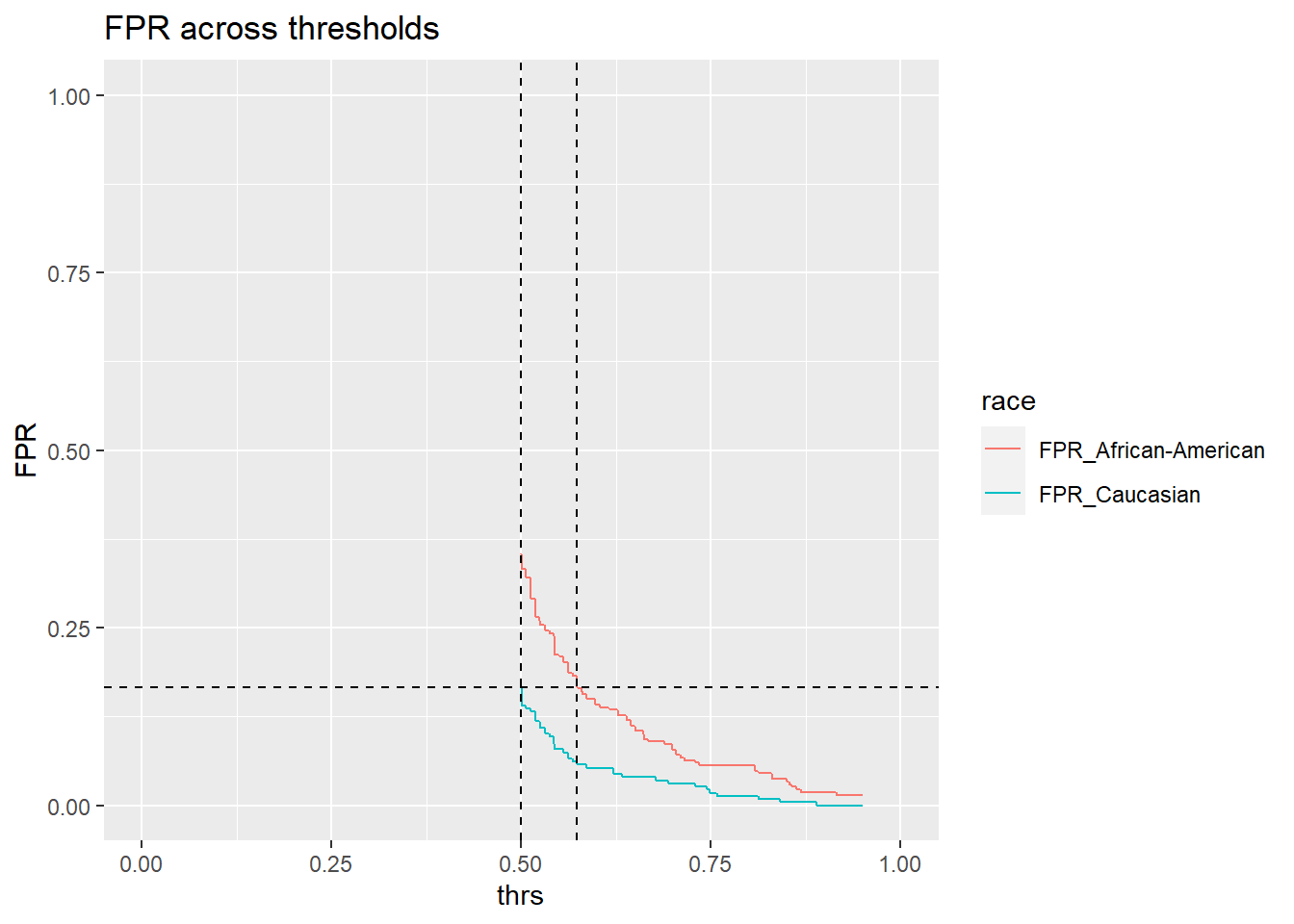

Threshold of 0.574 seems about right.

Now the two groups (Caucasian, African-American) would be at parity. We’ll compute the correct classification rate on data_analysis set (training set).

data_analysis.b <- data_analysis %>% filter(race == "African-American")
data_analysis.w <- data_analysis %>% filter(race == "Caucasian")

n.correct <- sum(data_analysis.b$is_recid == (predict(fit, newdata = data_analysis.b, type = "response") > threshold_African_American)) +
  sum(data_analysis.w$is_recid == (predict(fit, newdata = data_analysis.w, type = "response") > 0.5))
n.total <- nrow(data_analysis.b) + nrow(data_analysis.w)

n.correct / n.total

[1] 0.6494297

(Note that we ignored everyone who wasn’t white or black. That’s OK to do, but including other demographics (in any way you like) is OK too).

3.5 Exercise/Homework

• Above we discovered that certain ethnic groups (African-Americans) are treated unfairly by the COMPASS software (as well as or own simply ML model).
  • Please first take the time to read and understand of the lab above.
  • Then, please use the code to explore whether we can find similar patterns (unfairness) for other socio-demographic variables, namely sex and age_cat for the using our prediction model. You can use the models fitted above. Below you can find the distribution of in our data. Importantly, identifying whether there is unfairness across gender and age groups is enough for this exercise so the necessary code is in Section 3.2.

table(data$sex)

Female   Male 
  1395   5819 

table(data$age_cat)

        25 - 45 Greater than 45    Less than 25 
           4109            1576            1529 

4 All the code

# install.packages(pacman)
pacman::p_load(tidyverse,
               tidymodels,
               naniar,
               knitr,
               kableExtra)
data <- read_csv(sprintf("https://docs.google.com/uc?id=%s&export=download",
                         "1plUxvMIoieEcCZXkBpj4Bxw1rDwa27tj"))
# Split the data into training and test data
  data_split <- initial_split(data, prop = 0.80)
  data_split # Inspect

# Extract the two datasets
  data_train <- training(data_split)
  data_test <- testing(data_split) # Do not touch until the end!

# Further split the training data into analysis (training2) and assessment (validation) dataset 
  data_folds <- validation_split(data_train, prop = .80)
  data_folds # Inspect: We have only 1 fold!
  
# Extract analysis ("training data 2") and assessment (validation) data
  data_analysis <- analysis(data_folds$splits[[1]])
  dim(data_analysis)
  data_assessment <- assessment(data_folds$splits[[1]])
  dim(assessment)

fit <- glm(is_recid ~ age + priors_count, 
           family = binomial, 
           data = data_analysis)
#fit$coefficients
summary(fit)
# Function: False Positive Rate
get_FPR <- function(data_set, # Use assessment or test data here
                    outcome, # Specify outcome variable
                    probability_predicted, # Specify var containted pred. probs.
                    thr) { # Specify threshold
  return( # display results
    # Sum above threshold AND NOT recidivate
    sum((data_set %>% select(all_of(probability_predicted)) >= thr) &
      (data_set %>% select(all_of(outcome)) == 0))
    / # divided by
      # Sum NOT recividate
      sum(data_set %>% select(all_of(outcome)) == 0)
  )
}
# Share of people over the threshold that did not recidivate
# of all that did not recidivate (who got falsely predicted to
# recidivate)

# Q: Please explain the function below!

# Function: False Negative Rate
get_FNR <- function(data_set,
                    outcome,
                    probability_predicted,
                    thr) {
  return(
    sum((data_set %>% select(all_of(probability_predicted)) < thr) &
      (data_set %>% select(all_of(outcome)) == 1)) # ?
    /
      sum(data_set %>% select(all_of(outcome)) == 1)
  ) # ?
}

# Q: Explain the function below!
# Function: Correct Classification Rate
get_CCR <- function(data_set,
                    outcome,
                    probability_predicted,
                    thr) {
  return(
    mean((data_set %>% select(all_of(probability_predicted)) >= thr) # ?
    ==
      data_set %>% select(all_of(outcome)))
  ) # ?
}
kable(table(data$race),
      col.names = c("Race", "Frequency"))
data_assessment_all <- data_assessment %>%
  mutate(race = "All") %>% # replace grouping variable with constant
  nest(.by = "race")
data_assessment_groups_race <- data_assessment %>%
  nest(.by = "race")

data_assessment_groups <- bind_rows(
  data_assessment_all,
  data_assessment_groups_race
)
data_assessment_groups
data_assessment_groups %>%
  mutate(
    FPR = map_dbl(
      .x = data,
      ~ get_FPR(
        data_set = .x,
        outcome = "is_recid",
        probability_predicted = "decile_score",
        thr = 5
      )
    ),
    FNR = map_dbl(
      .x = data,
      ~ get_FNR(
        data_set = .x,
        outcome = "is_recid",
        probability_predicted = "decile_score",
        thr = 5
      )
    ),
    CCR = map_dbl(
      .x = data,
      ~ get_CCR(
        data_set = .x,
        outcome = "is_recid",
        probability_predicted = "decile_score",
        thr = 5
      )
    )
  ) %>%
  mutate_if(is.numeric, round, digits = 2)
# Add predictions to data
data_assessment <- data_assessment %>%
  mutate(prediction = predict(fit,
    newdata = .,
    type = "response"
  ))

data_assessment_all <- data_assessment %>%
  mutate(race = "All") %>% # replace grouping variable with constant
  nest(.by = "race")
data_assessment_groups_race <- data_assessment %>%
  nest(.by = "race")

data_assessment_groups <- bind_rows(
  data_assessment_all,
  data_assessment_groups_race
)


data_assessment_groups %>%
  mutate(
    FPR = map_dbl(
      .x = data,
      ~ get_FPR(
        data_set = .x,
        outcome = "is_recid",
        probability_predicted = "prediction",
        thr = 0.5
      )
    ),
    FNR = map_dbl(
      .x = data,
      ~ get_FNR(
        data_set = .x,
        outcome = "is_recid",
        probability_predicted = "prediction",
        thr = 0.5
      )
    ),
    CCR = map_dbl(
      .x = data,
      ~ get_CCR(
        data_set = .x,
        outcome = "is_recid",
        probability_predicted = "prediction",
        thr = 0.5
      )
    )
  ) %>%
  mutate_if(is.numeric, round, digits = 2)
# Define threshold values
thrs <- seq(0.5, 0.95, 0.01)

# Expand df with threshold values and calculate rates
data_assessment_groups %>%
  filter(race != "Native American") %>% # too few observations
  expand(nesting(race, data), thrs) %>%
  mutate(
    FPR = map2_dbl(
      .x = data,
      .y = thrs,
      ~ get_FPR(
        data_set = .x,
        outcome = "is_recid",
        probability_predicted = "prediction",
        thr = .y
      )
    ),
    FNR = map2_dbl(
      .x = data,
      .y = thrs,
      ~ get_FNR(
        data_set = .x,
        outcome = "is_recid",
        probability_predicted = "prediction",
        thr = .y
      )
    ),
    CCR = map2_dbl(
      .x = data,
      .y = thrs,
      ~ get_CCR(
        data_set = .x,
        outcome = "is_recid",
        probability_predicted = "prediction",
        thr = .y
      )
    )
  ) %>%
  pivot_longer(
    cols = FPR:CCR,
    names_to = "measure",
    values_to = "value"
  ) %>%
  ggplot(mapping = aes(
    x = thrs,
    y = value,
    color = measure
  )) +
  geom_smooth(
    se = F,
    method = "loess"
  ) +
  facet_wrap(~race) +
  labs(
    title = "FPR, FNR and CCR across ethnic groups and thresholds",
    x = "(Probability-) Thresholds",
    y = "Measurement values (see legend)",
    color = "Measure"
  )
# Define threshold values
thrs <- seq(0.5, 0.95, 0.0005)

comparison_thresholds <- data_assessment_groups %>%
  filter(race == "African-American" | race == "Caucasian") %>% # too few observations
  expand(nesting(race, data), thrs) %>%
  mutate(FPR = map2_dbl(
    .x = data,
    .y = thrs,
    ~ get_FPR(
      data_set = .x,
      outcome = "is_recid",
      probability_predicted = "prediction",
      thr = .y
    )
  )) %>%
  select(-data) %>%
  pivot_wider(
    names_from = "race",
    values_from = "FPR",
    names_prefix = "FPR_"
  )

comparison_thresholds %>%
  kable() %>%
  kable_styling("striped", full_width = T) %>%
  scroll_box(height = "200px")

# FPR caucasion at threshold 0.5
threshold_caucasian <- comparison_thresholds$FPR_Caucasian[comparison_thresholds$thrs == 0.5]
round(threshold_caucasian,3)

# Treshold needed for African-Americans to have similar FPR to Caucasians
threshold_African_American <- comparison_thresholds$thrs[which.min(abs(threshold_caucasian - comparison_thresholds$`FPR_African-American`))]
threshold_African_American
comparison_thresholds %>%
  pivot_longer(
    cols = `FPR_African-American`:FPR_Caucasian,
    names_to = "race",
    values_to = "FPR"
  ) %>%
  ggplot() +
  geom_line(
    mapping = aes(
      x = thrs,
      y = FPR,
      color = race
    ),
    method = "loess", se = F
  ) +
  geom_vline(xintercept = 0.5, linetype = "dashed") +
  geom_vline(xintercept = threshold_African_American, linetype = "dashed") +
  geom_hline(yintercept = threshold_caucasian, linetype = "dashed") +
  xlim(0, 1) +
  ylim(0, 1) +
  ggtitle("FPR across thresholds")
data_analysis.b <- data_analysis %>% filter(race == "African-American")
data_analysis.w <- data_analysis %>% filter(race == "Caucasian")

n.correct <- sum(data_analysis.b$is_recid == (predict(fit, newdata = data_analysis.b, type = "response") > threshold_African_American)) +
  sum(data_analysis.w$is_recid == (predict(fit, newdata = data_analysis.w, type = "response") > 0.5))
n.total <- nrow(data_analysis.b) + nrow(data_analysis.w)

n.correct / n.total
table(data$sex)
table(data$age_cat)

References

Lee, Claire S, Jeremy Du, and Michael Guerzhoy. 2020. “Auditing the COMPAS Recidivism Risk Assessment Tool: Predictive Modelling and Algorithmic Fairness in CS1.” In Proceedings of the 2020 ACM Conference on Innovation and Technology in Computer Science Education, 535–36. ITiCSE ’20. New York, NY, USA: Association for Computing Machinery.