ML modelling with tidymodels
Learning outcomes/objective: Learn…
- …introduction to
tidymodels. - …how we built a ML/predictive model and using the tidy_models.
1 Fundstücke/Finding(s)
- China Police Data Leak
- Pause Giant AI Experiments: An Open Letter
- “we must ask ourselves: Should we let machines flood our information channels with propaganda and untruth? Should we automate away all the jobs, including the fulfilling ones? Should we develop nonhuman minds that might eventually outnumber, outsmart, obsolete and replace us? Should we risk loss of control of our civilization? Such decisions must not be delegated to unelected tech leaders.”
- 2023 AI Index Report (Stanford university): Key takeaways
- Industry races ahead of academia.
- Performance saturation on traditional benchmarks.
- AI is both helping and harming the environment.
- The world’s best new scientist… AI?
- The number of incidents concerning the misuse of AI is rapidly rising (e.g., Zelenskyy deepfake, prisoner call monitoring)
- The demand for AI-related professional skills is increasing across virtually every American industrial sector.
- For the first time in the last decade, year-over-year private investment in AI decreased.
- While the proportion of companies adopting AI has plateaued, the companies that have adopted AI continue to pull ahead.
- Policymaker interest in AI is on the rise.
- Chinese citizens are among those who feel the most positively about AI products and services. Americans… not so much.
2 Tidymodels (1)
- See github website.
3 Tidymodels and packages
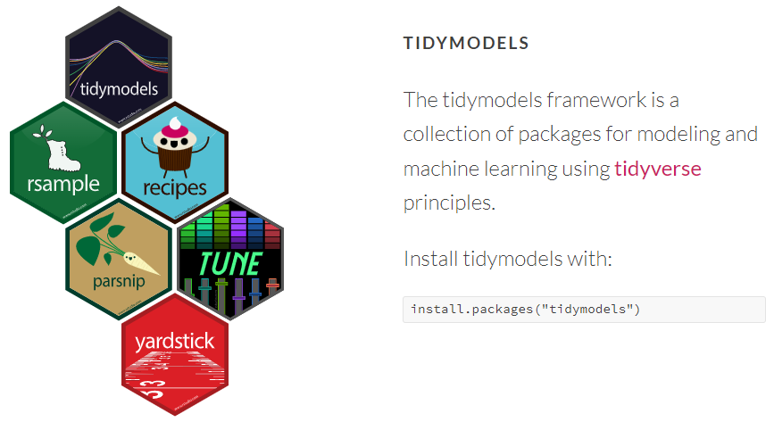
- A collection of packages for modeling and machine learning using tidyverse principles (see Barter (2020), Kuhn and Wickham (2020) and Kuhn and Silge (2022) for summaries)
- Much like
tidyverse,tidymodelsconsists of various core packages:rsample: for sample splitting (e.g. train/test or cross-validation)- Provides functions to create different types of resamples and corresponding classes for their analysis. The goal is to have a modular set of methods that can be used for resampling for estimating the sampling distribution of a statistic AND estimating model performance using a holdout set
prop-argument: Specify share of training data observationsstrata-argument: Conduct stratified sampling on the dependent variable (better if classes are imbalanced!)
recipes: for pre-processing- Use dplyr-like pipeable sequences of feature engineering steps to get your data ready for modeling.
parsnip: for specifying the model namely model type, engine and mode- Goal: provide a tidy, unified interface to access models from different packages
model type-argument: e.g, linear or logistic regressionengine-argument: R packages that contain these modelsmode-argument: either regression or classification
tune: for model tuning- Goal: facilitate hyperparameter tuning. It relies heavily on
recipes,parsnip, anddials.dials: contains infrastructure to create and manage values of tuning parameters
- Goal: facilitate hyperparameter tuning. It relies heavily on
yardstick: for evaluating the model- Goal: estimate how well models are working using tidy data principles
workflowsets:- Goal: allow users to create and easily fit a large number of different models.
- Use
workflowsetsto create aworkflow setthat holds multipleworkflow objects- These objects can be created by crossing all combinations of preprocessors (e.g., formula, recipe, etc) and model specifications. This set can be tuned or resampled using a set of specific functions.
4 The machine learning workflow using tidymodels
| Data resampling, feature engeneering | Model fitting, tuning | Model evaluation |
|---|---|---|
| rsample | tune | yardstick |
| recipes | parsnip | |
| dials |
- Different visualizations of the workflow
5 Lab: Using tidymodels to build a model to predict recidivism
5.1 Load the data
Below, we shortly assess how tidymodels could be used to built and evaluate our predictive model for recidivism relying on the rsample, parsnip and yardstick packages.
data <- read_csv(sprintf("https://docs.google.com/uc?id=%s&export=download",
                         "1plUxvMIoieEcCZXkBpj4Bxw1rDwa27tj"))
Then we create a factor version of is_recid that we label (so that we can look up what is what afterwards). We also order our variables differently.
data$is_recid <- factor(data$is_recid) # Convert to factor!)
data <- data %>% select(id, name, compas_screening_date, is_recid,
                        age, priors_count, everything())
5.2 rsample package: Split the data
# Split the data into training and test data
  data_split <- initial_split(data, prop = 0.80)
  data_split # Inspect
<Training/Testing/Total>
<5771/1443/7214># Extract the two datasets
data_train <- training(data_split)
data_test <- testing(data_split) # Do not touch until the end!
# Further split the training data into analysis (training2) and assessment (validation) dataset
data_folds <- validation_split(data_train, prop = .80)
data_folds # # We have only 1 fold!# Validation Set Split (0.8/0.2)
# A tibble: 1 x 2
splits id
<list> <chr>
1 <split [4616/1155]> validation# Extract analysis ("training data 2") and assessment (validation) data
data_analysis <- analysis(data_folds$splits[[1]])
data_assessment <- assessment(data_folds$splits[[1]])
dim(data_analysis)[1] 4616 53 dim(data_assessment)[1] 1155 535.3 parsnip package: Model specification using the parsnip package
# Define model with parsnip
lr_mod <- logistic_reg() %>% # Check out ?logistic_reg
set_engine('glm') %>% # Choose engine
set_mode('classification') # Choose mode
# Fit the model
fit <- lr_mod %>%
fit(is_recid ~ age + priors_count,
data = data_analysis)
# Check parameters
tidy(fit)# A tibble: 3 x 5
term estimate std.error statistic p.value
<chr> <dbl> <dbl> <dbl> <dbl>
1 (Intercept) 0.980 0.102 9.64 5.18e-22
2 age -0.0466 0.00297 -15.7 1.43e-55
3 priors_count 0.159 0.00843 18.9 1.94e-79# Obtain predictions (for )
predictions <- fit %>%
predict(new_data = data_assessment)
# Add predictions to dataset
data_assessment <- bind_cols(data_assessment,
predictions)
# Show predictions
data_assessment %>%
select(id, name, age, priors_count, is_recid, .pred_class)# A tibble: 1,155 x 6
id name age priors_count is_recid .pred_class
<dbl> <chr> <dbl> <dbl> <fct> <fct>
1 5063 monique howard 21 1 1 1
2 3015 jason gardner 46 1 1 0
3 8858 samuel mcleod 22 2 0 1
4 372 claire aspelly 40 3 0 0
5 9935 kevin soto 24 15 1 1
6 7697 owen parchment 29 0 0 0
7 7647 ronald knight 68 2 0 0
8 9703 trena collier 28 0 1 0
9 817 arrantes green 37 1 0 0
10 10649 marcus massicot 21 1 0 1
# ... with 1,145 more rows5.4 yardstick package: Evaluate model accuracy
conf_mat(): calculates a cross-tabulation of observed and predicted classes.metrics(): estimates one or more common performance estimates depending on the class of truth and returns them in a three column tibble.
conf_mat(data_assessment,
truth = is_recid,
estimate = .pred_class) # Beware of flipped rows/columns Truth
Prediction 0 1
0 460 194
1 153 348data_assessment %>%
metrics(truth = is_recid, estimate = .pred_class)# A tibble: 2 x 3
.metric .estimator .estimate
<chr> <chr> <dbl>
1 accuracy binary 0.700
2 kap binary 0.3945.5 Homework/Exercise:
Above we used a logistic regression model to predict recidivism. In principle, we could also use a linear probability model, i.e., estimate a linear regression and convert the predicted probabilities to a predicted binary outcome variable later on.
- What might be a problem when we use a linear probability model to obtain predictions (see James et al. (2013), Figure, 4.2, p. 131)?
- Please use the code above (see next section below) but now change the model to a linear probability model using the same variables. How is the accuracy of the lp-model as compared to the logistic model? Did you expect that?
- Tipps
- The linear probability model is defined through
linear_reg() %>% set_engine('lm') %>% set_mode('regression') - The linear probability model provides a predicted probability that needs to be converted to a binary class variable at the end.
- The linear probability model requires a numeric outcome, i.e., convert
is_recidonly to a factor at the end (as well as the predicted class).
- The linear probability model is defined through
6 All the code
data <- read_csv(sprintf("https://docs.google.com/uc?id=%s&export=download",
"1plUxvMIoieEcCZXkBpj4Bxw1rDwa27tj"))
data$is_recid <- factor(data$is_recid) # Convert to factor!)
data <- data %>% select(id, name, compas_screening_date, is_recid,
age, priors_count, everything())
# Split the data into training and test data
data_split <- initial_split(data, prop = 0.80)
data_split # Inspect
# Extract the two datasets
  data_train <- training(data_split)
  data_test <- testing(data_split) # Do not touch until the end!

# Further split the training data into analysis (training2) and assessment (validation) dataset
  data_folds <- validation_split(data_train, prop = .80)
  data_folds #   # We have only 1 fold!
# Extract analysis ("training data 2") and assessment (validation) data
  data_analysis <- analysis(data_folds$splits[[1]])
  data_assessment <- assessment(data_folds$splits[[1]])
  dim(data_analysis)
dim(data_assessment)
# Define model with parsnip
lr_mod <- logistic_reg() %>% # Check out ?logistic_reg
  set_engine('glm') %>% # Choose engine
  set_mode('classification') # Choose mode

# Fit the model
fit <- lr_mod %>%
  fit(is_recid ~ age + priors_count,
      data = data_analysis)

# Check parameters
tidy(fit)
# Obtain predictions (for )
predictions <- fit %>%
  predict(new_data = data_assessment)

# Add predictions to dataset
data_assessment <- bind_cols(data_assessment,
                             predictions)

# Show predictions
data_assessment %>%
  select(id, name, age, priors_count, is_recid, .pred_class)
conf_mat(data_assessment,
         truth = is_recid,
         estimate = .pred_class) # Beware of flipped rows/columns
data_assessment %>%
metrics(truth = is_recid, estimate = .pred_class)References
Barter, Rebecca. 2020. “Tidymodels: Tidy Machine Learning in R.” https://www.rebeccabarter.com/blog/2020-03-25_machine_learning/#what-is-tidymodels.
James, Gareth, Daniela Witten, Trevor Hastie, and Robert Tibshirani. 2013. An Introduction to Statistical Learning: With Applications in R. Springer Texts in Statistics. Springer.
Kuhn, M, and J Silge. 2022. “Tidy Modeling with R.”
Kuhn, M, and H Wickham. 2020. “Tidymodels: A Collection of Packages for Modeling and Machine Learning Using Tidyverse Principles.” Boston, MA, USA.