library(tidyverse)
library(tidymodels)

# Build and evaluate model without resampling
data <- read_csv(sprintf("https://docs.google.com/uc?id=%s&export=download",
"1azBdvM9-tDVQhADml_qlXjhpX72uHdWx"))Tree-based methods
Learning outcomes/objective: Learn…
- …what decision trees, bagging and random forests are.
- …how to use random forests in R.
Source(s): James et al. (2013, chap. 8); Tuning random forest hyperparameters with #TidyTuesday trees data
1 Fundstücke/Finding(s)
2 Supervised vs. unsupervised learning
- Supervised vs. unsupervised machine learning (James et al. 2013, 1; Athey and Imbens 2019, 689)
- Unsupervised statistical learning: There are inputs but no supervising output; we can still learn about relationships and structure from such data
- Only observe \(X_{i}\) and try to group them into clusters
- Supervised statistical learning: involves building a statistical model for predicting, or estimating, an output based on one or more inputs
- We observe both features \(x_{i}\) and the outcome \(y_{i}\)
- Use the model to predict unobserved outcomes \((y_{i})\) of units \(i\) where we only have \(x_{i}\)
- Unsupervised statistical learning: There are inputs but no supervising output; we can still learn about relationships and structure from such data
- Good analogy: Child in Kindergarden sorts toys (with or without teacher’s input)
3 Tree-based methods
- See James et al. (2013, chap. 8)
- “involve stratifying or segmenting the predictor space into a number of simple regions” (James et al. 2013, 303)
- Region: e.g., 2 variables and 2 cutoffs such as age (<25) and previous offenses (<1) → 4 regions/data subsets
- See James et al. (2013, 313), Figure 8.6.
- Outcome: Heart disease (Yes, No)
- Prediction for observation \(i\)
- Based on mean or mode (Q:?) of training observations in the region to which it belongs
- Decision tree methods: Name originates from splitting rules that can be summarized in a tree
- Can be applied to both regression and classification problems
- Predictive power of single decision tree not very good
- Bagging, random forests,and boosting
- Approaches involve producing multiple trees which are then combined to yield a single consensus prediction (“average prediction”)
- Combination of large number of trees can dramatically increase predictive power, but interpretation is more difficult (black box! Why?!)
4 Classification trees
- Predict qualitative outcomes rather than a quantitative one (vs. regression trees)
- Prediction: Unseen (test) observation \(i\) belongs to the most commonly occurring class of training observations (the mode) in the region to which it belongs
- Region: Young people (<25) with 3 previous offences
- Training observations: Most individuals in region re-offended
- Unseen/test observations: Prediction.. also re-offended
- To grow classification tree we use recursive splitting/partitioning
- Splitting training data into sub-populations based on several dichotomous independent variables
- Criterion for making binary splits: Classification error rate (vs. RSS in regression tree)
- minimize CRR: Fraction of training observations in region that do not belong to most common class in region
- \(E=1−\max\limits_{k}(\hat{p}_{mk})\) where \(\hat{p}_{mk}\) is proportion of training observations in the \(m\)th region that are from the \(k\)th class
- In practice: Use measures more sensitive to node purity, i.e., Gini index or cross-entropy (cf. James et al. 2013, 312)
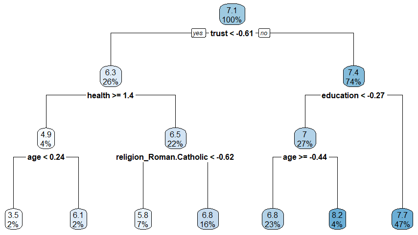
5 Regression tree
- Regression same logic as classification trees but use RSS as a criterion for making splits (+ min N of observations in final nodes/leaves)
- Figure 1 shows an exemplary tree based on our data (ESS: Predicting lifesatisfaction)
6 Advantages and Disadvantages of Trees (C.h 8.1.4)
- Pro
- Trees are very easy to explain to people (even easier than linear regression)!
- Decision trees more closely mirror human decision-making than do other regression and classification approaches
- Trees can be displayed graphically, and are easily interpreted even by a non-expert (especially if they are small).
- Trees can easily handle qualitative predictors without the need to create dummy variables.
- Contra
- Trees generally do not have the same level of predictive accuracy as some other regression and classification approaches in James et al. (2013).
- Trees can be very non-robust: a small change in the data can cause a large change in the final estimated tree.
7 Bagging
- Single decision trees may suffer from high variance, i.e., results could be very different for different splits
- Q: Why?
- We want: Low variance procedure that yields similar results if applied repeatedly to distinct training datasets (e.g., linear regression)
- Bagging: construct \(B\) regression trees using \(B\) bootstrapped training sets, and average the resulting predictions
- Bootstrap (also called bootstrap aggregation): Take repeated samples from the (single) training set, built predictive model and average predictions
- Classification: For a given test observation, we can record the class predicted by each of the \(B\) trees, and take a majority vote: the overall prediction is the most commonly occurring majority vote class among the \(B\) predictions
- Regression problem: Average across \(B\) predictions
8 Out-of-Bag (OOB) Error Estimation
- Out-of-Bag (OBB) Error estimation: Straightforward way to estimate test error of bagged model (no need for cross-validation)
- On average each bagged tree makes use of around two-thirds of the observations
- remaining one-third of observations not used to fit a given bagged tree are referred to as the out-of-bag (OOB) observations
- Predict outcome for the \(i\)th observation using each of the trees in which that observation was OOB
- Will yield around \(B/3\) predictions for the \(i\)th observation
- Then average these predicted responses (if regression is the goal) or take a majority vote (if classification is the goal)
- Leads to a single OOB prediction for the \(i\)th observation
- OOB prediction can be obtained in this way for each of the \(n\) observations, from which the overall OOB classification error can be computed (Regression: OOB MSE)
- Resulting OOB error is a valid estimate of the test error for the bagged model
- Because outcome/response for each observation is predicted using only the trees that were not fit using that observation
- It can be shown that with \(B\) sufficiently large, OOB error is virtually equivalent to leave-one-out cross-validation error.
- OOB test error approach particularly convenient for large data sets for which cross-validation would be computationally onerous
9 Variable Importance Measures
- Variable importance: Which are the most important predictors?
- Single decision tree: Intepretation is easy.. just look at the splits in the graph
- e.g., Figure 1 or Figure 8.6. (James et al. 2013, 313) lower right Thalium stress test (Tahl) is most important
- Bag of large number of trees: Can’t just visualize single tree and no longer clear which variables are most relevant for splits
- Bagging improves prediction accuracy at the expense of interpretability (James et al. 2013, 319)
- Overall summary of importance of each predictor
- Using Gini index (measure of node purity) for bagging classification trees (or RSS for regression trees)
- Classification trees: Add up the total amount that the Gini index is decreased (i.e., node purity increased) by splits over a given predictor, averaged over all \(B\) trees
- Gini index: a small value indicates that a node contains predominantly observations from a single class
- See Figure 8.9 (James et al. 2013, 313) for graphical representation of importance: Mean decrease in Gini index for each variable relative to the largest
- Classification trees: Add up the total amount that the Gini index is decreased (i.e., node purity increased) by splits over a given predictor, averaged over all \(B\) trees
- Using Gini index (measure of node purity) for bagging classification trees (or RSS for regression trees)
10 Random forests
- Random Forests (RFs) provide improvement over bagged trees
- Decorrelated trees lead to reduction in both test and OOB error over bagging
- RFs also build decision trees on bootstrapped training samples but…
- ….add predictor subsetting:
- Each time a split in a tree is considered,a random sample of \(m\) predictors is chosen as split candidates from the full set of \(p\) predictors
- Split only allowed to use one of \(m\) predictors
- Fresh sample of \(m\) predictors taken at each split (typically not all but \(m \approx \sqrt{p}\)!)
- On average \((p-m)/p\) splits won’t consider strong predictor (decorrelating trees)
- Objective: Avoid that single strong predictor is always used for first split & decrease correlation of trees
- Main difference bagging vs. random forests: Choice of predictor subset size \(m\)
- RF built using \(m=p\) equates Bagging
- Recommmendation: Vary \(m\) and use small \(m\) when predictors are highly correlated
- Finally, boosting (skipped here) grows trees sequentially using information from previous trees ee Chapter 8.2.3 (James et al. 2013, 321)
11 Lab: Tree-based methods & random forests
Section 11.1 discusses the steps underlying prediction using random forest (RF) models WITHOUT tuning. Section 11.2 discusses the steps underlying prediction using random forest (RF) models WITH tuning.
Below the steps we would pursue WITHOUT tuning in Section 11.1.
- Step 1: Load data, recode and rename variables
- Step 2: Split the data (training vs. test data)
- Step 3: Specify recipe, model and workflow
- Step 4: Evaluate model using resampling
- Step 5: Fit final model to training data
- Step 6: Fit final model to test data and assess accuracy
When tuning in Section 11.2 we can re-use Step 1 and Step 2 from Section 11.1. However, the rest of the steps slighlty differ.
- Step 3: Specify recipe, model, workflow and tuning parameters
- Step 4: Tune, evaluate the model using resampling and choose the best model
- Step 5: Fit final model to training data
- Step 6: Fit final model to test data and assess accuracy
11.1 Random forest (without tuning)
11.1.1 Step 1: Loading, renaming and recoding
We’ll use the ESS data that we have used in the previous lab. The variables were not named so well, so we have to rely on the codebook to understand their meaning. You can find it here or on the website of the ESS.
stflife: measures life satisfaction (How satisfied with life as a whole).uempla: measures unemployment (Doing last 7 days: unemployed, actively looking for job).uempli: measures life satisfaction (Doing last 7 days: unemployed, not actively looking for job).eisced: measures education (Highest level of education, ES - ISCED).cntry: measures a respondent’s country of origin (here held constant for France).- etc.
We first import the data into R:
Below we recode missings and also rename some of our variables (for easier interpretation later on):
data <- data  %>%
    filter(cntry=="FR") %>% # filter french respondents
 # Recode missings
 mutate(ppltrst = if_else(ppltrst %in% c(55, 66, 77, 88, 99), NA, ppltrst),
        eisced = if_else(eisced %in% c(55, 66, 77, 88, 99), NA, eisced),
        stflife = if_else(stflife %in% c(55, 66, 77, 88, 99), NA, stflife)) %>%
 # Rename variables
 rename(country = cntry,
        unemployed_active = uempla,
        unemployed = uempli,
        trust = ppltrst,
        lifesatisfaction = stflife,
        education = eisced,
        age = agea,
        religion = rlgdnm,
        children_number = chldo12) %>% # we add this variable
  mutate(religion = factor(recode(religion, # Recode and factor
    "1" = "Roman Catholic",
    "2" = "Protestant",
    "3" = "Eastern Orthodox",
    "4" = "Other Christian denomination",
    "5" = "Jewish",
    "6" = "Islam",
    "7" = "Eastern religions",
    "8" = "Other Non-Christian religions",
    .default = NA_character_))) %>%
  select(idno,
         lifesatisfaction,
        unemployed_active,
        unemployed,
        trust,
        lifesatisfaction,
        education,
        age,
        religion,
        health,
        children_number)  %>%
  drop_na(education, trust) %>%
  filter(!is.na(lifesatisfaction))
kable(head(data))| idno | lifesatisfaction | unemployed_active | unemployed | trust | education | age | religion | health | children_number |
|---|---|---|---|---|---|---|---|---|---|
| 10005 | 10 | 0 | 0 | 5 | 4 | 23 | Roman Catholic | 2 | 0 |
| 10007 | 7 | 0 | 0 | 7 | 6 | 32 | NA | 2 | 0 |
| 10011 | 7 | 0 | 0 | 5 | 4 | 25 | NA | 2 | 0 |
| 10022 | 5 | 0 | 0 | 7 | 1 | 74 | Roman Catholic | 4 | 0 |
| 10025 | 7 | 0 | 0 | 4 | 4 | 39 | Roman Catholic | 2 | 0 |
| 10050 | 10 | 0 | 0 | 3 | 3 | 59 | NA | 3 | 2 |
11.1.2 Step 2: Split the data (training vs. test data)
Below we split the data and create resampled partitions with vfold_cv() stored in an object called data_folds. Hence, we have the original data_train and data_test but also already resamples of data_train in data_folds.
# Split the data into training and test data
  data_split <- initial_split(data, prop = 0.80)
  data_split # Inspect
<Training/Testing/Total>
<1568/392/1960># Extract the two datasets
data_train <- training(data_split)
data_test <- testing(data_split) # Do not touch until the end!
# Create resampled partitions
set.seed(345)
data_folds <- vfold_cv(data_train, v = 10) # V-fold/k-fold cross-validation
data_folds # data_folds now contains several resamples of our training data # 10-fold cross-validation
# A tibble: 10 x 2
splits id
<list> <chr>
1 <split [1411/157]> Fold01
2 <split [1411/157]> Fold02
3 <split [1411/157]> Fold03
4 <split [1411/157]> Fold04
5 <split [1411/157]> Fold05
6 <split [1411/157]> Fold06
7 <split [1411/157]> Fold07
8 <split [1411/157]> Fold08
9 <split [1412/156]> Fold09
10 <split [1412/156]> Fold10 # You can also try loo_cv(data_train) instead11.1.3 Step 3: Specify recipe, model and workflow
Below we define different pre-processing steps in our recipe (see # comments):
# Define recipe
model_recipe <-
recipe(formula = lifesatisfaction ~ ., data = data_train) %>%
step_naomit(all_predictors()) %>%
update_role(idno, new_role = "id vars") %>% # declare ID variables
step_nzv(all_predictors(), freq_cut = 0, unique_cut = 0) %>% # remove variables with zero variances
step_novel(all_nominal_predictors()) %>% # prepares data to handle previously unseen factor levels
step_unknown(all_nominal_predictors()) %>% # categorizes missing categorical data (NA's) as `unknown`
step_dummy(all_nominal_predictors(), -has_role("id vars")) %>% # dummy codes categorical variables
step_zv(all_predictors()) %>% # remove vars with only single value
step_normalize(all_predictors()) # normale predictorsThen we specify our RF model choosing a mode, engine and specifying the workflow with workflow():
# Specify model
set.seed(100)
model_rf <-
rand_forest(trees = 1000) %>% # grow 1000 trees!
set_engine("ranger",
importance = "permutation") %>%
set_mode("regression")
# Specify workflow
wflow_rf <-
workflow() %>%
add_recipe(model_recipe) %>%
add_model(model_rf)11.1.4 Step 4: Evaluate model using resampling
Then we fit the RF to our resamples of the training data (different splits into analysis and assessment data) to be better able to evaluate it accounting for possible variation across subsets:
# Fit the random forest to the cross-validation datasets
fit_rf <- fit_resamples(
object = wflow_rf,
resamples = data_folds,
metrics = metric_set(rmse, rsq, mae),
control = control_resamples(verbose = TRUE, # show live comments
save_pred = TRUE, # save predictions
extract = function(x) extract_model(x))) # save modelsAnd we can evaluate the metrics:
# RMSE and RSQ
collect_metrics(fit_rf)# A tibble: 3 x 6
.metric .estimator mean n std_err .config
<chr> <chr> <dbl> <int> <dbl> <chr>
1 mae standard 1.64 10 0.0362 Preprocessor1_Model1
2 rmse standard 2.12 10 0.0541 Preprocessor1_Model1
3 rsq standard 0.103 10 0.0146 Preprocessor1_Model1Q: What do the different variables stand for?
We can also collect the average predictions (these are averaged across the folds):
assessment_data_predictions <- collect_predictions(fit_rf, summarize = TRUE)
assessment_data_predictions# A tibble: 1,568 x 4
.row lifesatisfaction .config .pred
<int> <dbl> <chr> <dbl>
1 1 3 Preprocessor1_Model1 7.55
2 2 8 Preprocessor1_Model1 6.75
3 3 5 Preprocessor1_Model1 6.93
4 4 9 Preprocessor1_Model1 7.16
5 5 10 Preprocessor1_Model1 7.42
6 6 6 Preprocessor1_Model1 6.59
7 7 9 Preprocessor1_Model1 6.71
8 8 8 Preprocessor1_Model1 7.69
9 9 8 Preprocessor1_Model1 7.82
10 10 10 Preprocessor1_Model1 7.17
# ... with 1,558 more rows
Visualization also sometimes makes sense to identify outliers that are not well predicted by the model. Figure 2 provides a quick graph that may serve to start a discussion in which regions of the outcome/reponse variable our predictive model is off.
Q: Can you interpret the graph?
assessment_data_predictions %>%
ggplot(aes(x = lifesatisfaction, y = .pred)) +
geom_point(alpha = .15) +
geom_abline(color = "red") +
coord_obs_pred() +
ylab("Life satisfaction: Predicted values") +
xlab("Life satisfaction: Actual values")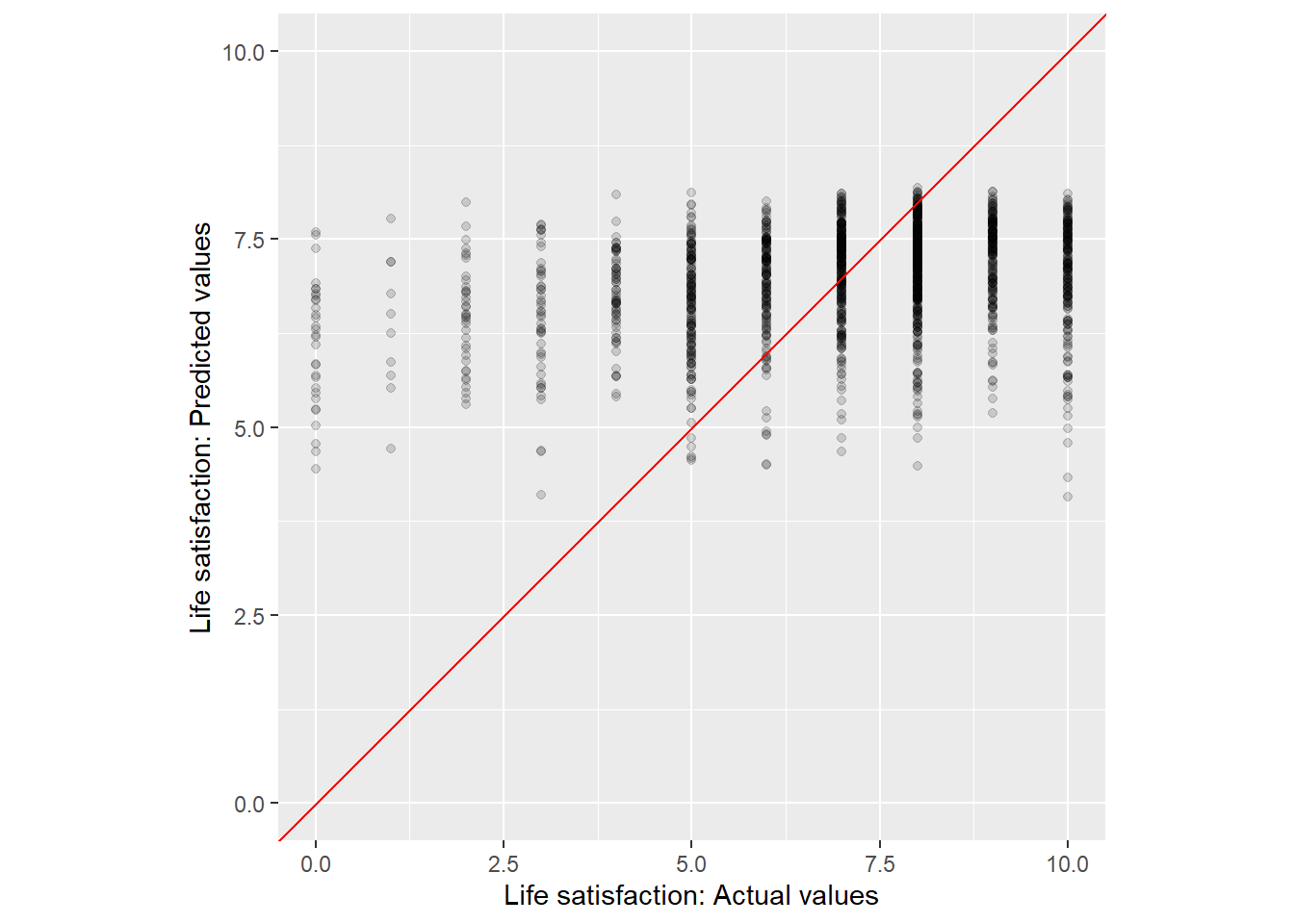
11.1.5 Step 5: Fit final model to training data
Once we we are happy with our random forest model (after having used resampling to assess it and potential alternatives) we can fit our workflow that includes the model to the complete training data data_train and also assess it’s accuracy for the training data again.
# Fit the model
rf_final_fit <- fit(wflow_rf, data = data_train)
# Check accuracy in for complete training data
augment(rf_final_fit, new_data = data_train) %>%
mae(truth = lifesatisfaction, estimate = .pred)# A tibble: 1 x 3
.metric .estimator .estimate
<chr> <chr> <dbl>
1 mae standard 1.46
Now, we can also explore the variable importance of different predictors and visualize it in Figure 3. The vip() does only like objects of class ranger, hence we have to directly access ist in the layer object using rf_final_fit$fit$fit$fit
# install.packages("vip")
library(vip)
rf_final_fit$fit$fit$fit %>%
vip::vip(geom = "point")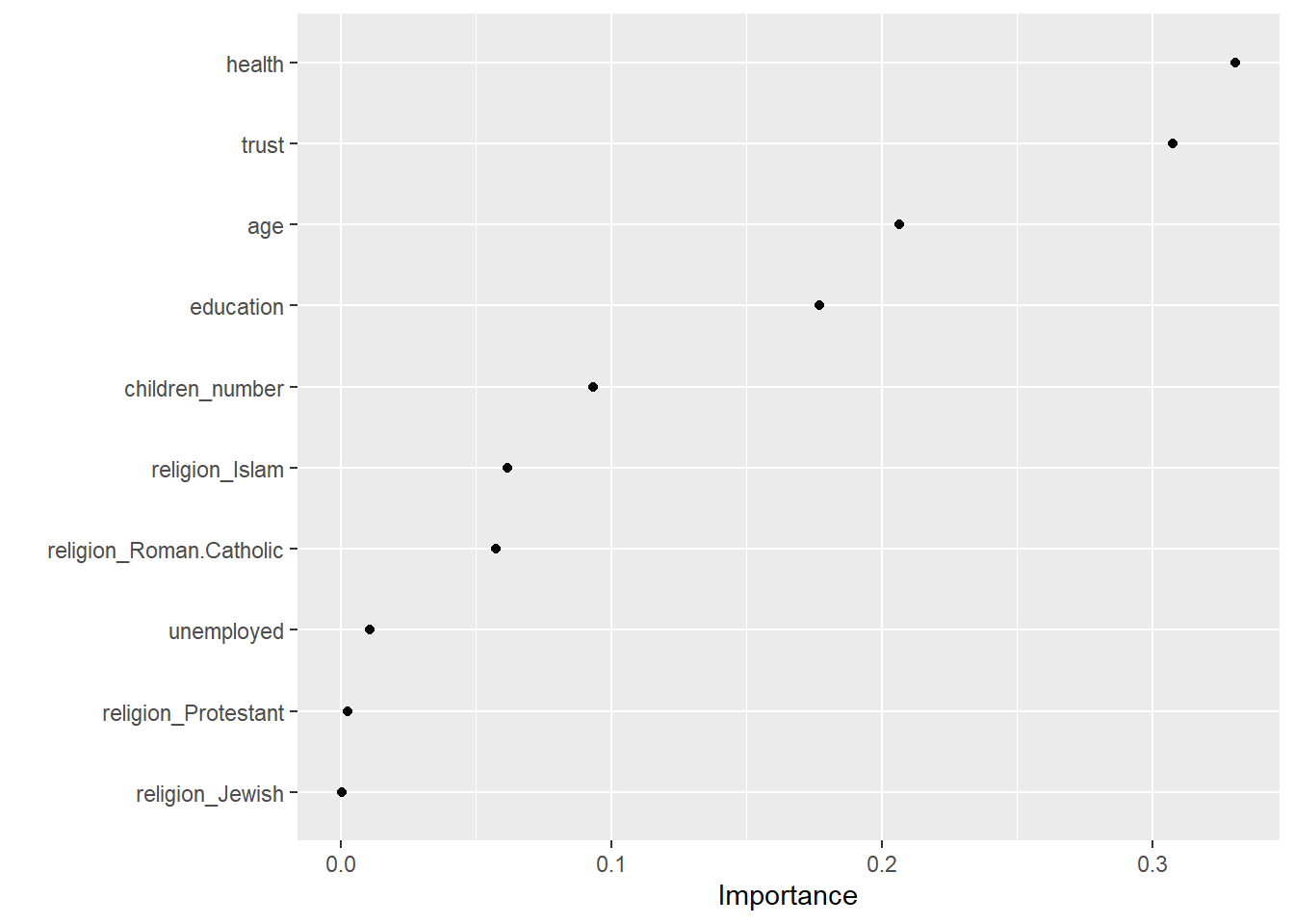
Q: What do we see here?
11.1.6 Step 6: Fit final model to test data and assess accuracy
We then use the model rf_final_fit fitted/trained on the training data and evaluate the accuracy of this model which is based on the training data using the test data data_test. We use augment() to obtain the predictions:
# Use fitted model to predict values
augment(rf_final_fit, new_data = data_test)# A tibble: 392 x 11
idno lifesatisf~1 unemp~2 unemp~3 trust educa~4 age relig~5 health child~6
<dbl> <dbl> <dbl> <dbl> <dbl> <dbl> <dbl> <fct> <dbl> <dbl>
1 10050 10 0 0 3 3 59 <NA> 3 2
2 10096 6 0 0 0 5 51 <NA> 3 2
3 10155 9 0 0 5 5 36 Roman ~ 1 0
4 10159 5 0 0 3 3 84 <NA> 2 2
5 10196 8 0 0 6 7 44 Roman ~ 2 1
6 10210 8 0 0 5 3 53 Roman ~ 2 1
7 10278 7 0 0 5 3 42 <NA> 2 0
8 10299 6 0 0 7 3 53 Roman ~ 3 1
9 10321 8 0 0 7 1 83 <NA> 2 3
10 10341 9 0 0 4 5 47 Roman ~ 3 2
# ... with 382 more rows, 1 more variable: .pred <dbl>, and abbreviated
# variable names 1: lifesatisfaction, 2: unemployed_active, 3: unemployed,
# 4: education, 5: religion, 6: children_number
And can directly pipe the result into functions such as rsq(), rmse() and mae() to obtain the corresponding measures of accuracy in the test data data_test.
augment(rf_final_fit, new_data = data_test) %>%
rsq(truth = lifesatisfaction, estimate = .pred)# A tibble: 1 x 3
.metric .estimator .estimate
<chr> <chr> <dbl>
1 rsq standard 0.135augment(rf_final_fit, new_data = data_test) %>%
rmse(truth = lifesatisfaction, estimate = .pred)# A tibble: 1 x 3
.metric .estimator .estimate
<chr> <chr> <dbl>
1 rmse standard 2.01augment(rf_final_fit, new_data = data_test) %>%
mae(truth = lifesatisfaction, estimate = .pred)# A tibble: 1 x 3
.metric .estimator .estimate
<chr> <chr> <dbl>
1 mae standard 1.56Q: How does our model compare to the accuracy from the ridge and lasso regression models?
11.1.7 Extracting information on a single
Importantly, sometimes we might want to extract one or several trees from our random forest. This can be done by directly accessing the corresponding sub-elements in the corresponding object. For ?@tbl-tree we extracted the corresponding information using the treeInfo() function that works for ranger objects where tree = 1 is the first tree. See ?treeInfo for a description of the different variables. Unfortunately, there is not convenient plotting function atm.
tree_table <- treeInfo(rf_final_fit$fit$fit$fit, tree = 1)
kable(head(tree_table))?(caption)
| nodeID | leftChild | rightChild | splitvarID | splitvarName | splitval | terminal | prediction |
|---|---|---|---|---|---|---|---|
| 0 | 1 | 2 | 2 | trust | -0.5880124 | FALSE | NA |
| 1 | 3 | 4 | 8 | religion_Islam | 0.9556334 | FALSE | NA |
| 2 | 5 | 6 | 5 | health | -0.8353954 | FALSE | NA |
| 3 | 7 | 8 | 4 | age | 0.2459335 | FALSE | NA |
| 4 | 9 | 10 | 5 | health | -0.8353954 | FALSE | NA |
| 5 | 11 | 12 | 11 | religion_Other.Non.Christian.religions | 6.1686775 | FALSE | NA |
Variable importance for different predictors
That table indicates that the first split happended on the following variable/value:
trust: -0.59.
11.2 Random forest (with tuning)
Here, we can re-use Step 1 and Step 2 from Section 11.1.
11.2.1 Step 3: Specify recipe, model, workflow and tuning parameters
Similar to ridge or lasso regression a random forest has parameters that we can try to tune. Below, we create a model specification for a RF where we will tune…
mtrythe number of predictors to sample at each split andmin_nthe number of observations needed in each resulting node to keep splitting.
These are hyperparameters that can’t be learned from data when training the model. (cf. Source)
# Specify model with tuning
model_rf <- rand_forest(
mtry = tune(), # tune mtry parameter
trees = 1000, # grow 1000 trees
min_n = tune() # tune min_n parameter
) %>%
set_mode("regression") %>%
set_engine("ranger",
importance = "permutation") # potentially computational intensive
# Specify workflow (with tuning)
workflow_rf <- workflow() %>%
add_recipe(model_recipe) %>%
add_model(model_rf)11.2.2 Step 4: Tune, evaluate the model using resampling and choose/explore the best model
11.2.2.1 Tune, evaluate the model using resampling
Below we use tune_grid() to compute performance metrics (e.g. accuracy or RMSE) for pre-defined set of tuning parameters that correspond to a model or recipe across one or more resamples of the data (below 10 stored in data_folds).
# Specify to use parallel processing
doParallel::registerDoParallel()
set.seed(345)
tune_result <- tune_grid(
workflow_rf,
resamples = data_folds,
grid = 20 # choose 20 grid points automatically
)
tune_result# Tuning results
# 10-fold cross-validation
# A tibble: 10 x 4
splits id .metrics .notes
<list> <chr> <list> <list>
1 <split [1411/157]> Fold01 <tibble [40 x 6]> <tibble [0 x 3]>
2 <split [1411/157]> Fold02 <tibble [40 x 6]> <tibble [0 x 3]>
3 <split [1411/157]> Fold03 <tibble [40 x 6]> <tibble [0 x 3]>
4 <split [1411/157]> Fold04 <tibble [40 x 6]> <tibble [0 x 3]>
5 <split [1411/157]> Fold05 <tibble [40 x 6]> <tibble [0 x 3]>
6 <split [1411/157]> Fold06 <tibble [40 x 6]> <tibble [0 x 3]>
7 <split [1411/157]> Fold07 <tibble [40 x 6]> <tibble [1 x 3]>
8 <split [1411/157]> Fold08 <tibble [40 x 6]> <tibble [0 x 3]>
9 <split [1412/156]> Fold09 <tibble [40 x 6]> <tibble [0 x 3]>
10 <split [1412/156]> Fold10 <tibble [40 x 6]> <tibble [0 x 3]>
There were issues with some computations:
- Warning(s) x1: 14 columns were requested but there were 13 predictors in the dat...
Run `show_notes(.Last.tune.result)` for more information.
Visualizing the results helps us to evaluate the tuning results. Figure 4 indicates that higher values of min_n and lower values of mtry seem to work better in terms of accuracy.
tune_result %>%
collect_metrics() %>% # extract metrics
filter(.metric == "rmse") %>% # keep rmse only
select(mean, min_n, mtry) %>% # subset variables
pivot_longer(min_n:mtry, # convert to longer
values_to = "value",
names_to = "parameter"
) %>%
ggplot(aes(value, mean, color = parameter)) + # plot!
geom_point(show.legend = FALSE) +
facet_wrap(~parameter, scales = "free_x") +
labs(x = NULL, y = "RMSE")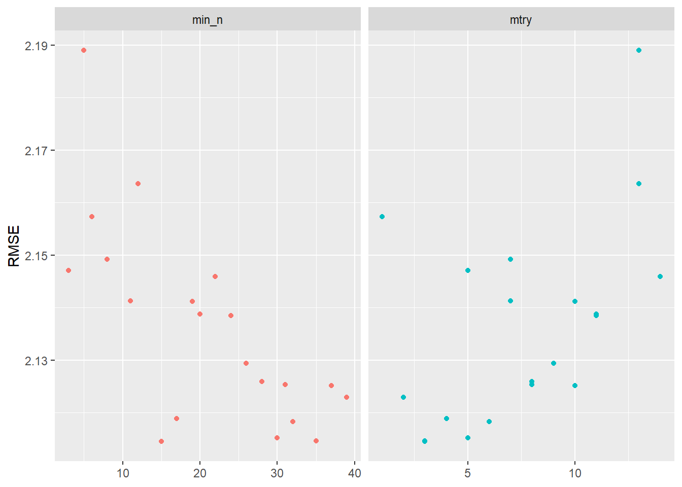
After getting this first glimpse in Figure 4 we might want to make further changes to the grid values that we use for tuning. Below we pick ranges that turned out to be better in Figure 4:
rf_grid <- grid_regular(
mtry(range = c(0, 10)), # define range for mtry
min_n(range = c(20, 40)), # define range for min_n
levels = 6 # number of values of each parameter to use to make the regular grid
)
rf_grid# A tibble: 36 x 2
mtry min_n
<int> <int>
1 0 20
2 2 20
3 4 20
4 6 20
5 8 20
6 10 20
7 0 24
8 2 24
9 4 24
10 6 24
# ... with 26 more rowsThen we re-do the tuning using those values:
set.seed(456)
tune_result2 <- tune_grid(
workflow_rf,
resamples = data_folds,
grid = rf_grid
)
tune_result2# Tuning results
# 10-fold cross-validation
# A tibble: 10 x 4
splits id .metrics .notes
<list> <chr> <list> <list>
1 <split [1411/157]> Fold01 <tibble [72 x 6]> <tibble [0 x 3]>
2 <split [1411/157]> Fold02 <tibble [72 x 6]> <tibble [0 x 3]>
3 <split [1411/157]> Fold03 <tibble [72 x 6]> <tibble [0 x 3]>
4 <split [1411/157]> Fold04 <tibble [72 x 6]> <tibble [0 x 3]>
5 <split [1411/157]> Fold05 <tibble [72 x 6]> <tibble [0 x 3]>
6 <split [1411/157]> Fold06 <tibble [72 x 6]> <tibble [0 x 3]>
7 <split [1411/157]> Fold07 <tibble [72 x 6]> <tibble [0 x 3]>
8 <split [1411/157]> Fold08 <tibble [72 x 6]> <tibble [0 x 3]>
9 <split [1412/156]> Fold09 <tibble [72 x 6]> <tibble [0 x 3]>
10 <split [1412/156]> Fold10 <tibble [72 x 6]> <tibble [0 x 3]>Again we visualize the results in Figure 5:
tune_result2 %>%
collect_metrics() %>%
filter(.metric == "rmse") %>%
select(mean, min_n, mtry) %>%
pivot_longer(min_n:mtry,
values_to = "value",
names_to = "parameter"
) %>%
ggplot(aes(value, mean, color = parameter)) +
geom_point(show.legend = FALSE) +
facet_wrap(~parameter, scales = "free_x") +
labs(x = NULL, y = "RMSE")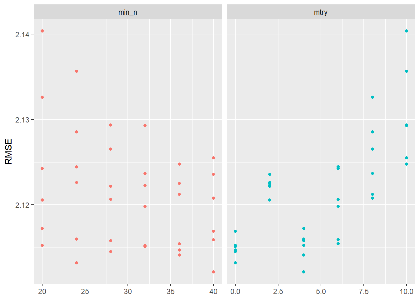
11.2.2.2 Choose best model after tuning
Choosing the best model, i.e., the model with the best parameter choices obtained in the tuning above (tune_result2), can be done with the select_best() function. After having selected the best parameter values, we update our original model specification stored in model_rf using the finalize_model() function.
# Find tuning parameter combination with best performance values
best_rmse <- select_best(tune_result2, "rmse")
# Take list/tibble of tuning parameter values
# and update model_rf with those values.
final_rf_specification <- finalize_model(
model_rf,
best_rmse # define
)11.2.3 Step 5: Fit final model to training data and assess accuracy
Once we are happy with our tuned random forest model and have chosen the best model specification stored in final_rf_specification we can fit our workflow to the training data data_train again and also assess it’s accuracy again.
# Define final workflow
final_wf <- workflow() %>%
add_recipe(model_recipe) %>% # use standard recipe
add_model(final_rf_specification) # use final model
# Fit the model
rf_final_fit <- fit(final_wf, data = data_train)
rf_final_fit== Workflow [trained] ==========================================================
Preprocessor: Recipe
Model: rand_forest()
-- Preprocessor ----------------------------------------------------------------
7 Recipe Steps
* step_naomit()
* step_nzv()
* step_novel()
* step_unknown()
* step_dummy()
* step_zv()
* step_normalize()
-- Model -----------------------------------------------------------------------
Ranger result
Call:
ranger::ranger(x = maybe_data_frame(x), y = y, mtry = min_cols(~4L, x), num.trees = ~1000, min.node.size = min_rows(~40L, x), importance = ~"permutation", num.threads = 1, verbose = FALSE, seed = sample.int(10^5, 1))
Type: Regression
Number of trees: 1000
Sample size: 777
Number of independent variables: 14
Mtry: 4
Target node size: 40
Variable importance mode: permutation
Splitrule: variance
OOB prediction error (MSE): 3.859915
R squared (OOB): 0.09845296 # Q: What do the values for `mtry` and `min_n` in the final model mean?
# Check accuracy in training data using MAE
augment(rf_final_fit, new_data = data_train) %>%
mae(truth = lifesatisfaction, estimate = .pred)# A tibble: 1 x 3
.metric .estimator .estimate
<chr> <chr> <dbl>
1 mae standard 1.54
Now, that we have our final model we can also explore it assessing variable importance (i.e., which variables where the most relevant to find splits) using the vip package. We can use vi() and vip() to extract or extract+plot the variable importance of different predictors as shown in ?@tbl-vip and Figure 6. The vi() and vip() function does only like objects of class ranger, hence we have to directly access is in the layer object using rf_final_fit$fit$fit$fit
# install.packages("vip")
library(vip)
rf_final_fit$fit$fit %>%
vip::vi() %>%
kable()?(caption)
| Variable | Importance |
|---|---|
| trust | 0.3152158 |
| health | 0.3150181 |
| education | 0.1624100 |
| age | 0.1478958 |
| religion_Islam | 0.0506248 |
| religion_Roman.Catholic | 0.0499890 |
| children_number | 0.0397902 |
| unemployed | 0.0093475 |
| religion_Protestant | 0.0027482 |
| religion_Eastern.religions | 0.0000000 |
| religion_Other.Christian.denomination | -0.0008228 |
| religion_Other.Non.Christian.religions | -0.0012179 |
| religion_Jewish | -0.0034335 |
| unemployed_active | -0.0035191 |
Variable importance for different predictors
rf_final_fit$fit$fit %>%
vip(geom = "point")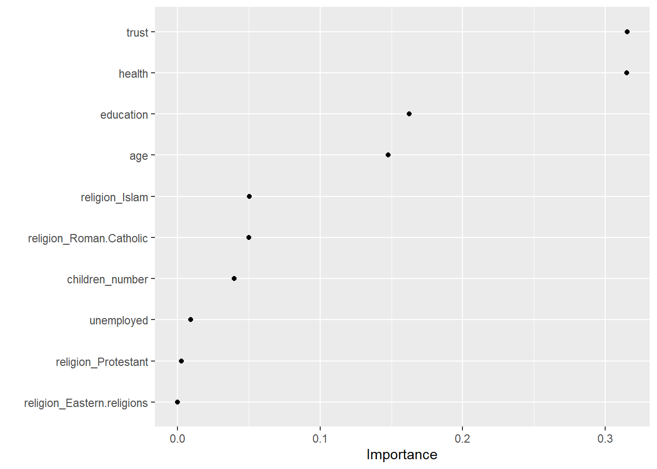
11.2.4 Step 6: Fit final model to test data and assess accuracy
We then evaluate the accuracy of this model which is based on the training data using the test data data_test. We use augment() to obtain the predictions:
# Use fitted model to predict values
augment(rf_final_fit, new_data = data_test)# A tibble: 392 x 11
idno lifesatisf~1 unemp~2 unemp~3 trust educa~4 age relig~5 health child~6
<dbl> <dbl> <dbl> <dbl> <dbl> <dbl> <dbl> <fct> <dbl> <dbl>
1 10050 10 0 0 3 3 59 <NA> 3 2
2 10096 6 0 0 0 5 51 <NA> 3 2
3 10155 9 0 0 5 5 36 Roman ~ 1 0
4 10159 5 0 0 3 3 84 <NA> 2 2
5 10196 8 0 0 6 7 44 Roman ~ 2 1
6 10210 8 0 0 5 3 53 Roman ~ 2 1
7 10278 7 0 0 5 3 42 <NA> 2 0
8 10299 6 0 0 7 3 53 Roman ~ 3 1
9 10321 8 0 0 7 1 83 <NA> 2 3
10 10341 9 0 0 4 5 47 Roman ~ 3 2
# ... with 382 more rows, 1 more variable: .pred <dbl>, and abbreviated
# variable names 1: lifesatisfaction, 2: unemployed_active, 3: unemployed,
# 4: education, 5: religion, 6: children_number
And can directly pipe the result into functions such as rsq(), rmse() and mae() to obtain the corresponding measures of accuracy in the test data data_test.
augment(rf_final_fit, new_data = data_test) %>%
rsq(truth = lifesatisfaction, estimate = .pred)# A tibble: 1 x 3
.metric .estimator .estimate
<chr> <chr> <dbl>
1 rsq standard 0.135augment(rf_final_fit, new_data = data_test) %>%
rmse(truth = lifesatisfaction, estimate = .pred)# A tibble: 1 x 3
.metric .estimator .estimate
<chr> <chr> <dbl>
1 rmse standard 2.01augment(rf_final_fit, new_data = data_test) %>%
mae(truth = lifesatisfaction, estimate = .pred)# A tibble: 1 x 3
.metric .estimator .estimate
<chr> <chr> <dbl>
1 mae standard 1.5512 All the code
library(tidyverse)
library(tidymodels)
library(knitr)
data <- readr::read_csv("ESS10.csv")
library(tidyverse)
library(tidymodels)
# Build and evaluate model without resampling
data <- read_csv(sprintf("https://docs.google.com/uc?id=%s&export=download",
"1azBdvM9-tDVQhADml_qlXjhpX72uHdWx"))
data <- data %>%
filter(cntry=="FR") %>% # filter french respondents
# Recode missings
mutate(ppltrst = if_else(ppltrst %in% c(55, 66, 77, 88, 99), NA, ppltrst),
eisced = if_else(eisced %in% c(55, 66, 77, 88, 99), NA, eisced),
stflife = if_else(stflife %in% c(55, 66, 77, 88, 99), NA, stflife)) %>%
# Rename variables
rename(country = cntry,
unemployed_active = uempla,
unemployed = uempli,
trust = ppltrst,
lifesatisfaction = stflife,
education = eisced,
age = agea,
religion = rlgdnm,
children_number = chldo12) %>% # we add this variable
mutate(religion = factor(recode(religion, # Recode and factor
"1" = "Roman Catholic",
"2" = "Protestant",
"3" = "Eastern Orthodox",
"4" = "Other Christian denomination",
"5" = "Jewish",
"6" = "Islam",
"7" = "Eastern religions",
"8" = "Other Non-Christian religions",
.default = NA_character_))) %>%
select(idno,
lifesatisfaction,
unemployed_active,
unemployed,
trust,
lifesatisfaction,
education,
age,
religion,
health,
children_number) %>%
drop_na(education, trust) %>%
filter(!is.na(lifesatisfaction))
kable(head(data))
# Split the data into training and test data
data_split <- initial_split(data, prop = 0.80)
data_split # Inspect
# Extract the two datasets
  data_train <- training(data_split)
  data_test <- testing(data_split) # Do not touch until the end!

# Create resampled partitions
  set.seed(345)
  data_folds <- vfold_cv(data_train, v = 10) # V-fold/k-fold cross-validation
  data_folds # data_folds now contains several resamples of our training data
# You can also try loo_cv(data_train) instead
# Define recipe
model_recipe <-
  recipe(formula = lifesatisfaction ~ ., data = data_train) %>%
  step_naomit(all_predictors()) %>%
  update_role(idno, new_role = "id vars") %>% # declare ID variables
  step_nzv(all_predictors(), freq_cut = 0, unique_cut = 0) %>% # remove variables with zero variances
  step_novel(all_nominal_predictors()) %>% # prepares data to handle previously unseen factor levels
  step_unknown(all_nominal_predictors()) %>% # categorizes missing categorical data (NA's) as `unknown`
  step_dummy(all_nominal_predictors(), -has_role("id vars")) %>% # dummy codes categorical variables
  step_zv(all_predictors()) %>% # remove vars with only single value
  step_normalize(all_predictors()) # normale predictors
# Specify model
set.seed(100)
model_rf <-
  rand_forest(trees = 1000) %>% # grow 1000 trees!
  set_engine("ranger",
             importance = "permutation") %>%
  set_mode("regression")

# Specify workflow
wflow_rf <-
  workflow() %>%
  add_recipe(model_recipe) %>%
  add_model(model_rf)
#
# tree <- decision_tree() %>%
# set_engine("rpart") %>%
# set_mode("regression")
#
# tree_wf <- workflow() %>%
# add_recipe(model_recipe) %>%
# add_model(tree) %>%
# fit(data_train) #results are found here
#
# tree_fit <- tree_wf %>%
# pull_workflow_fit()
# rpart.plot(tree_fit$fit)
# Store manually: 10_01_figure_tree.png
# Fit the random forest to the cross-validation datasets
fit_rf <- fit_resamples(
  object = wflow_rf,
  resamples = data_folds,
  metrics = metric_set(rmse, rsq, mae),
  control = control_resamples(verbose = TRUE, # show live comments
                              save_pred = TRUE, # save predictions
                              extract = function(x) extract_model(x))) # save models
# RMSE and RSQ
collect_metrics(fit_rf)
assessment_data_predictions <- collect_predictions(fit_rf, summarize = TRUE)
assessment_data_predictions
assessment_data_predictions %>%
  ggplot(aes(x = lifesatisfaction, y = .pred)) +
  geom_point(alpha = .15) +
  geom_abline(color = "red") +
  coord_obs_pred() +
  ylab("Life satisfaction: Predicted values") +
  xlab("Life satisfaction: Actual values")
# Fit the model
rf_final_fit <- fit(wflow_rf, data = data_train)

# Check accuracy in for complete training data
  augment(rf_final_fit, new_data = data_train) %>%
    mae(truth = lifesatisfaction, estimate = .pred)
# install.packages("vip")
library(vip)
rf_final_fit$fit$fit$fit %>%
    vip::vip(geom = "point")
# Use fitted model to predict values
  augment(rf_final_fit, new_data = data_test)
augment(rf_final_fit, new_data = data_test) %>%
  rsq(truth = lifesatisfaction, estimate = .pred)
augment(rf_final_fit, new_data = data_test) %>%
  rmse(truth = lifesatisfaction, estimate = .pred)
augment(rf_final_fit, new_data = data_test) %>%
    mae(truth = lifesatisfaction, estimate = .pred)
tree_table <- treeInfo(rf_final_fit$fit$fit$fit, tree = 1)
kable(head(tree_table))
x <- tree_table %>% select(splitvarName, splitval) %>%
slice(1) %>%
mutate(splitval = round(splitval,2)) %>%
unite("splitvarName_splitval",
splitvarName:splitval,
sep=": ") %>%
dplyr::summarise(splitvarName_splitval = paste(splitvarName_splitval,
collapse = ", ")) %>%
pull(splitvarName_splitval)
# Specify model with tuning
model_rf <- rand_forest(
  mtry = tune(), # tune mtry parameter
  trees = 1000, # grow 1000 trees
  min_n = tune() # tune min_n parameter
) %>%
  set_mode("regression") %>%
  set_engine("ranger",
             importance = "permutation") # potentially computational intensive


# Specify workflow (with tuning)
workflow_rf <- workflow() %>%
  add_recipe(model_recipe) %>%
  add_model(model_rf)
# Specify to use parallel processing
doParallel::registerDoParallel()

set.seed(345)
tune_result <- tune_grid(
  workflow_rf,
  resamples = data_folds,
  grid = 20 # choose 20 grid points automatically
)

tune_result
tune_result %>%
  collect_metrics() %>% # extract metrics
  filter(.metric == "rmse") %>% # keep rmse only
  select(mean, min_n, mtry) %>% # subset variables
  pivot_longer(min_n:mtry, # convert to longer
    values_to = "value",
    names_to = "parameter"
  ) %>%
  ggplot(aes(value, mean, color = parameter)) + # plot!
  geom_point(show.legend = FALSE) +
  facet_wrap(~parameter, scales = "free_x") +
  labs(x = NULL, y = "RMSE")
rf_grid <- grid_regular(
  mtry(range = c(0, 10)), # define range for mtry
  min_n(range = c(20, 40)), # define range for min_n
  levels = 6 # number of values of each parameter to use to make the regular grid
)

rf_grid
set.seed(456)
tune_result2 <- tune_grid(
  workflow_rf,
  resamples = data_folds,
  grid = rf_grid
)

tune_result2
tune_result2 %>%
  collect_metrics() %>%
  filter(.metric == "rmse") %>%
  select(mean, min_n, mtry) %>%
  pivot_longer(min_n:mtry,
    values_to = "value",
    names_to = "parameter"
  ) %>%
  ggplot(aes(value, mean, color = parameter)) +
  geom_point(show.legend = FALSE) +
  facet_wrap(~parameter, scales = "free_x") +
  labs(x = NULL, y = "RMSE")
# Find tuning parameter combination with best performance values
best_rmse <- select_best(tune_result2, "rmse")

# Take list/tibble of tuning parameter values
# and update model_rf with those values.
final_rf_specification <- finalize_model(
  model_rf,
  best_rmse # define
)
# Define final workflow
final_wf <- workflow() %>%
  add_recipe(model_recipe) %>% #  use standard recipe
  add_model(final_rf_specification) # use final model

# Fit the model
rf_final_fit <- fit(final_wf, data = data_train)
rf_final_fit
# Q: What do the values for `mtry` and `min_n` in the final model mean?

# Check accuracy in training data using MAE
  augment(rf_final_fit, new_data = data_train) %>%
    mae(truth = lifesatisfaction, estimate = .pred)
# install.packages("vip")
library(vip)
rf_final_fit$fit$fit %>%
    vip::vi() %>%
  kable()
rf_final_fit$fit$fit %>%
  vip(geom = "point")
# Use fitted model to predict values
  augment(rf_final_fit, new_data = data_test)
augment(rf_final_fit, new_data = data_test) %>%
  rsq(truth = lifesatisfaction, estimate = .pred)
augment(rf_final_fit, new_data = data_test) %>%
  rmse(truth = lifesatisfaction, estimate = .pred)
augment(rf_final_fit, new_data = data_test) %>%
    mae(truth = lifesatisfaction, estimate = .pred)
labs = knitr::all_labels()
ignore_chunks <- labs[str_detect(labs, "exclude|setup|solution|get-labels")]
labs = setdiff(labs, ignore_chunks)References
Athey, Susan, and Guido W Imbens. 2019. “Machine Learning Methods That Economists Should Know About.” Annu. Rev. Econom. 11 (1): 685–725.
James, Gareth, Daniela Witten, Trevor Hastie, and Robert Tibshirani. 2013. An Introduction to Statistical Learning: With Applications in R. Springer Texts in Statistics. Springer.