| idno | Name | Country | Trust | Education | Unemployed | Unemployed_active |
|---|---|---|---|---|---|---|
| 10005 | Lamar | FR | 5 | 4 | 0 | 0 |
| 10608 | Darren | FR | 5 | 3 | 1 | 0 |
| 10007 | Matthew | FR | 7 | 6 | 0 | 0 |
| 10751 | Brandon | FR | 5 | 3 | 0 | 1 |
| 11170 | Jenna | FR | 0 | NA | 1 | 0 |
| 10405 | Brenna | FR | 0 | NA | 0 | 1 |
| .. | .. | .. | .. | .. | .. | .. |
Predictive models
Learning outcomes/objective: Learn…
- …and repeat logic underlying models.
- …that there is a (joint-)distribution underlying and model.
- …concepts (training dataset, accuracy etc.) using a “simple example”.
1 Fundstücke/Finding(s)
2 Mean as a ‘predictive model’
2.1 Mean as a model: Data (1)
- Data: European Social Survey (ESS): Round 10 - 2020. Democracy, Digital social contacts
- Measures of trust, unemployment etc.
- Q: Are the names in Table 1 real?
- We will use this data shown in Table 1 for our prediction challenge later on!
2.2 Mean as a model (2)
- Model(s) = Mathematical equation(s)
- Underlying a model is always a (joint) distribution
- Model summarizes (joint) distribution with fewer parameters
- e.g. mean with one parameter
- e.g., linear model with three variables (\(y\), \(x1\), \(x2\)) with three parameters (\(\text{intercept }\beta + \beta_{1} + \beta_{2}\))
- …we start with a simple example!
- “using only information from the outcome variable itself for our prediction”
2.3 Mean as a model (3)
- Simple model: Mean of the distribution of a variable
\[ \begin{aligned} Trust_{Claudia} = 5 = \underbrace{\color{blue}{\overline{y}}}_{\color{green}{\widehat{y}}_{Claudia}} \pm \color{red}{\varepsilon}_{Claudia} = \color{blue}{4.7} + \color{red}{0.3} \end{aligned} \]
Mean (= model) predicts Claudia’s value with a certain error
Q: How well does the model (mean = 4.7) predict person’s that have values of 1, of 4.7 or of 8?
Important: We could use this model – this mean – to predict…
- …trust values of people that gave no answer (missings in the dataset)
- …trust values of another group of people
- …future trust values of other or the same people
Here the outcome variable has values from 0-10. The mean for a binary outcome variable is simply the share of 1s, e.g., in the data above the share (mean) of unemployed actively looking for a job (France) is 0.04 (73 out of 1977).
2.4 Mean as a model (table) (4)
- In Table 2 we added our predictions to the data showing only the first ten lines of the dataset (see column “error”)
- Mean provides same prediction \((\hat{y})\) for everyone
| Name | Country | Trust | prediction (mean) | error |
|---|---|---|---|---|
| Jazmin | FR | 5 | 4.687 | 0.313 |
| Khaila | FR | 7 | 4.687 | 2.313 |
| Bradley | FR | 5 | 4.687 | 0.313 |
| Exaviah | FR | 7 | 4.687 | 2.313 |
| Ashley | FR | 4 | 4.687 | -0.687 |
| Jennifer | FR | 3 | 4.687 | -1.687 |
| Lindsey | FR | 4 | 4.687 | -0.687 |
| Quinn | FR | 6 | 4.687 | 1.313 |
- Q1: What are the (dis-)advantages of taking the mean as a predictive model? Is it a good predictive model?
- Q2: How could we assess whether the mean is a good predictive model? Do we need training and test data for that?
- Q3: In how for does the data determine whether the mean is a good predictive model?
Answer
- Q1
- Advantages: Simple, fast, works with sparse information (outcome only)
- Disadvantages: Potentially very biased/large errors
- Q2
- We can calculate the mean error \(\overline{\color{red}{\varepsilon}}\)
- \(\bar{\varepsilon} = \frac{\varepsilon_{1}+\varepsilon_{2}+\cdots +\varepsilon_{n}}{n}=\frac{\sum_{i}^{n} \varepsilon_{i}}{n}\)
- -0.00042
- Why is the error close to 0? Why is it not 0?
- We can calculate the mean error \(\overline{\color{red}{\varepsilon}}\)
- Q3
- Mean can be very good if everyone lies close to the mean (e.g., mean age is 25 whereby all students are between 24 and 26 years old)
3 Training, validation and test dataset (1)
- As shown in Figure 2 when training models we sometimes…
- …only split into one training data subset (e.g., 80% of observations) and one test data subset (e.g., 20% of observations)
- … introduce one further split
- e.g., built models on training (analysis) dataset, validate/tune model using validation (assessment) dataset and use test dataset ONLY for final test
- As indicated in Figure 2, Plot 3 when doing further splitting the training data we use the terms analysis and assessment dataset (Kuhn and Johnson 2019) (see also next slide)
- e.g., built models on training (analysis) dataset, validate/tune model using validation (assessment) dataset and use test dataset ONLY for final test
- …do resampling, i.e., repeatedly splitting the data (more on that later!)
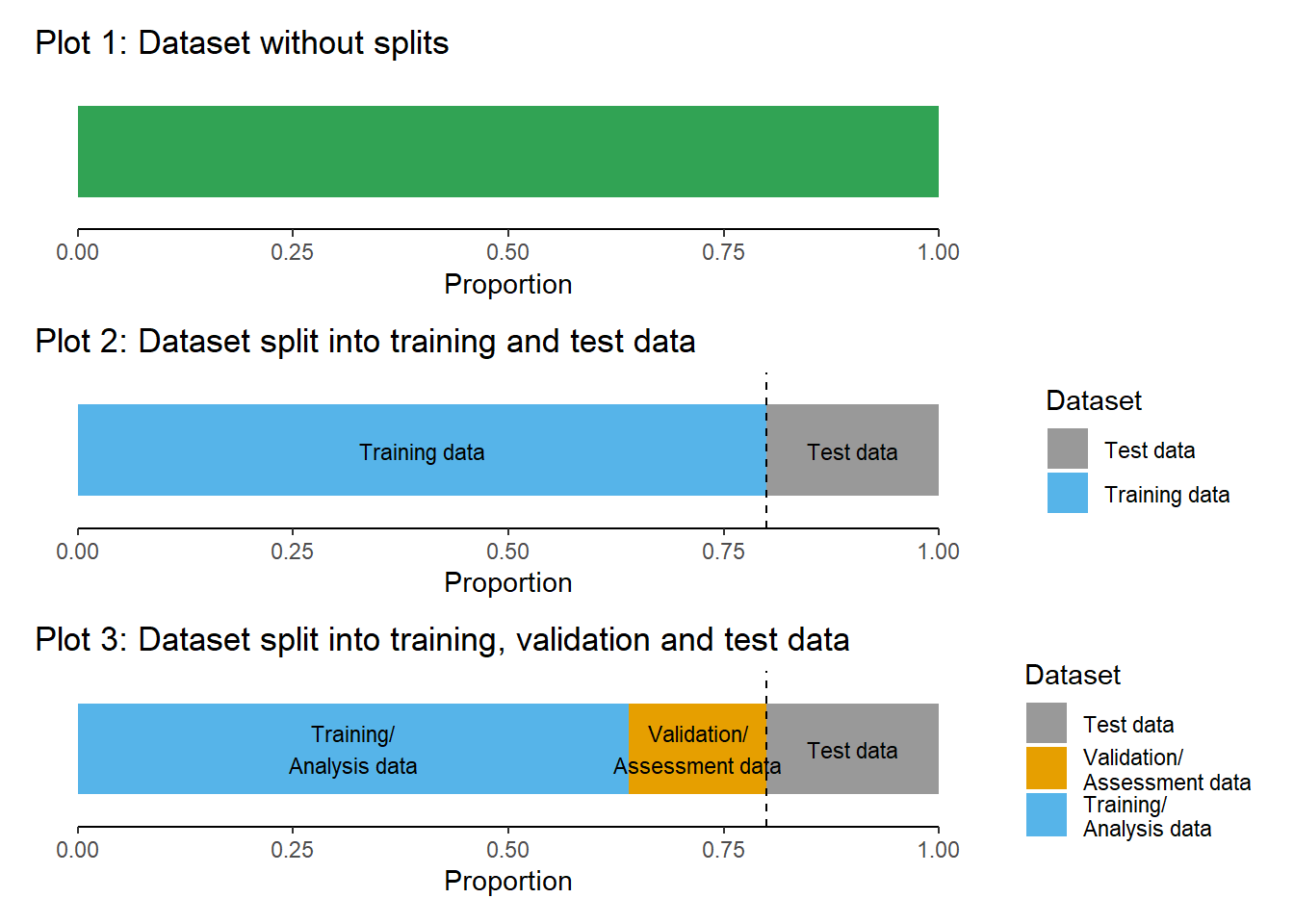
4 Training, validation and test dataset (2)
- To avoid conceptual confusion we use the terminology by Kuhn and Johnson (2019) and illustrated in Figure Figure 3
- Datasets obtained from the initial split are called training and test data
- Datasets obtained from further splits to the training data are called analysis and assessment datasets
- Often such further splits are called folds.

5 Training, validation and test dataset (3)
- Size of datasets: Usually 80/20 splits but depends..
- Q: What could be a problem if training and/or test dataset is too small?
Answer
- Training data ↓ → Variance of parameter estimates ↑
- Test data ↓ → Variance of performance statistic ↑
5.1 Mean as ML model? (5)
- If we were to follow a machine learning logic we would proceed as follows:
- Step 1: Split data shown in Figure 1 into two subsets: training and test data
- Step 2: Train model, i.e., calculate the mean of trust for training dataset
- Step 3: Check accuracy of model in training dataset (calculate the average error)
- Step 4: Check accuracy in test dataset (calculate the average error)
- Step 5: If happy we could use our model (trust mean from training dataset) to predict, e.g., missings in the data on the variable trust
  # install.packages("rsample")
  library(rsample)

# Load dataset
  # data <- read_csv(sprintf("https://docs.google.com/uc?id=%s&export=download",
  #                          "1bQlc8MxRU5eIywlIJhL7BVLKWlyhvjVZ"))
  data <- readr::read_csv("www/data_ess_prepared.csv")

# Set seed
  set.seed(42) # Why?


# Step 1
# Create a split object (?initial_split)
  data_split <- initial_split(data, prop = 0.80)
  data_split
<Training/Testing/Total>
<1581/396/1977># Extract training dataframe
data_training <- training(data_split)
# Extract test dataframe
data_test <- testing(data_split)
# Check dimensions of the two datasets
dim(data_training)[1] 1581 9 dim(data_test)[1] 396 9# Step 2
trust_mean_model <- mean(data_training$Trust, na.rm=TRUE)
# Step 3
data_training <- data_training %>%
mutate(prediction = trust_mean_model) %>% # Append predictions
mutate(error = trust_mean_model - Trust)
mean(data_training$error, na.rm=TRUE) # Check accuracy in training data[1] 0.0000000000000001782972# Step 4
data_test <- data_test %>%
mutate(prediction = trust_mean_model) %>% # Append predictions
mutate(error = trust_mean_model - Trust)
mean(data_test$error) # # Check accuracy in training data[1] -0.03194388 # Is that ok? Hard to tell!
# Mean model predicts the same values (y^) for every individual
# Step 5: Repeat steps 1-4 until happy!6 Stratified splitting
- Stratified splitting: involves preserving the class distribution in each split of the dataset.
- We may use it to preserve class representation, i.e., assure the sample representativity of each class after splitting which has several advantages (-> generalization, reliable evaluation, enhanced model fairness, consistent experimentation and comparison)1
Show the code
library(tidyverse)
library(tidymodels)

# Build and evaluate model without resampling
data <- read_csv(sprintf("https://docs.google.com/uc?id=%s&export=download",
                         "1azBdvM9-tDVQhADml_qlXjhpX72uHdWx"))
Show the code
data <- data  %>%
    filter(cntry=="FR") %>% # filter french respondents
 # Recode missings
 mutate(ppltrst = if_else(ppltrst %in% c(55, 66, 77, 88, 99), NA, ppltrst),
        eisced = if_else(eisced %in% c(55, 66, 77, 88, 99), NA, eisced),
        stflife = if_else(stflife %in% c(55, 66, 77, 88, 99), NA, stflife)) %>%
 # Rename variables
 rename(country = cntry,
        unemployed_active = uempla,
        unemployed = uempli,
        trust = ppltrst,
        lifesatisfaction = stflife,
        education = eisced,
        age = agea,
        religion = rlgdnm,
        children_number = chldo12) %>% # we add this variable
  mutate(religion = factor(recode(religion, # Recode and factor
    "1" = "Roman Catholic",
    "2" = "Protestant",
    "3" = "Eastern Orthodox",
    "4" = "Other Christian denomination",
    "5" = "Jewish",
    "6" = "Islam",
    "7" = "Eastern religions",
    "8" = "Other Non-Christian religions",
    .default = NA_character_))) %>%
  select(idno,
         lifesatisfaction,
        unemployed_active,
        unemployed,
        trust,
        lifesatisfaction,
        education,
        age,
        religion,
        health,
        children_number)  %>%
  drop_na(education, trust) %>%
filter(!is.na(lifesatisfaction)) set.seed(123) # Why?
# Split the data into training and test data
data_split <- initial_split(data, prop = 0.8, strata = unemployed)
data_split # Inspect<Training/Testing/Total>
<1568/392/1960> round(prop.table(table(training(data_split)$unemployed)), 3) # not perfect...| 0 | 1 |
|---|---|
| 0.981 | 0.019 |
round(prop.table(table(testing(data_split)$unemployed)), 3)| 0 | 1 |
|---|---|
| 0.99 | 0.01 |
strata = ...: A variable used to conduct stratified sampling. When not NULL, each resample is created within the stratification variable. Numeric strata are binned into quartiles.- This can help ensure that the resample(s) has/have equivalent proportions as the original data set.
- For a categorical variable, sampling is conducted separately within each class.
- For a numeric stratification variable, strata is binned into quartiles, which are then used to stratify. Strata below 10% of the total are pooled together
- This can help ensure that the resample(s) has/have equivalent proportions as the original data set.
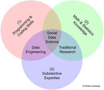
7 Predictive modelling: Skills
8 Prediction: Model (general form)
- cf. James et al. (2013, 16–21)
- Output variable \(Y\), e.g., life satistfaction, trust, unemployment, recidivism
- Often called the response/dependent variable
- Input variable(s) \(X\) (usually with subscript, e.g., \(X_{1}\) is education)
- Usually called predictors/independent variables/features
- Example
- Quantitative response \(Y\) and \(p\) different predictors, \(X_{1},...,X_{p}\)
- We assume a relationship between output \(Y\) and inputs \(X = X_{1},...,X_{p}\)
- can be written generally as \(Y = f(X) + \varepsilon\)
- \(f\) represents the systematic information that \(X\) provides about \(Y\)
- \(\varepsilon\) is a random error term which is independent of \(X\) and has mean zero
- can be written generally as \(Y = f(X) + \varepsilon\)
9 Prediction: Why estimate \(f\) (model)?
Pertains to class distinction discussed in (Breiman 2001; James et al. 2013, 17–19)
Prediction: In many situations, a set of inputs \(X\) readily available, but output \(Y\) cannot be easily obtained
- In this setting, since the error term averages to zero, we can predict \(Y\) using \(\hat{Y} = \hat{f}(X)\)
- where \(\hat{f}\) represents our estimate for \(f\), and \(\hat{Y}\) represents the resulting prediction for \(Y\)
- \(f\) is “true” function that produced \(Y\), e.g., “true” function/model that produces unemployment
- \(f\) is often treated as a black box, i.e., typically we are less concerned with exact form of \(\hat{f}\) provided that the predictions are accurate
- In this setting, since the error term averages to zero, we can predict \(Y\) using \(\hat{Y} = \hat{f}(X)\)
Inference: Understand the relationship between \(Y\) and \(X\) (see corresponding questions in James et al. (2013, 19–20))
10 Prediction: Accuracy
- Accuracy of \(\hat{Y}\) as prediction for \(Y\) depends on two quantities
- reducible error (introduced by innaccuracy of \(\hat{f}\)) and the irreducible error (associated with \(\varepsilon\))
- \(\hat{f}\) will not be a perfect estimate of \(f\) but introduce error
- This error is reducible because we can potentially improve the accuracy of \(\hat{f}\) by using the most appropriate statistical learning technique to estimate \(f\)
- But even with perfect estimate of \(f\) (estimate response with form \(\hat{Y} = f (X)\)) error remains because \(Y\) is also function of \(\varepsilon\) that cannot be predicted using \(X\)
- Variability associated with \(\varepsilon\) also affects predictions and is called irreducible error
- Q: Why is the irreproducible error (always) larger than 0?
Answer
The quantity \(\varepsilon\) may contain unmeasured variables that are useful in predicting \(Y\): since we don’t measure them, \(f\) cannot use them for its prediction. The quantity may also contain unmeasurable variation (James et al. 2013, 18–19).
Irreducible error will always provide an upper bound on the accuracy of our prediction for Y. This bound is almost always unknown in practice since we may not have measured/know the necessary features/predictors. (James et al. 2013, 19)
11 Prediction: How Do We Estimate f?
We estimate \(f\) using the training data (James et al. 2013, 21–24)
Parametric methods with two-step approach (James et al. 2013, 21–24)
- Make assumption about the functional form of \(f\), or shape, e.g., linear model
- Train or fit the model, e.g., most common method for linear model is (ordinary) least squares
- “parametric” because assumpions about data distribution (e.g., linear) and reduces problem of estimating \(f\) down to estimating a set of parameters, e.g., coefficients of linear model
- Potential disadvantage: the model we choose will usually not match the true unknown form of \(f\).. if too far from true \(f\) then estimate will be poor
- Flexible models can fit many different function forms for \(f\) but require estimating more parameters but increase danger of overfitting (Q: Overfitting?)
Non-parametric methods (e.g. random forests)
- Do not make explicit assumptions about the functional form of \(f\)
- Seek estimate of \(f\) that gets as close to the data points as possible without being too rough or wiggly
12 Trade-Off(s): Prediction Accuracy vs. Model Interpretability
- Some ML methods are more some are less flexible (shape of f)
- James et al. (2013, 25), Fig. 2.7. provides an overview
- Q: Why would we ever choose to use a more restrictive method (less flexible) model instead of a very flexible approach?
Answer
- Inference: If main goal is inference, restrictive models are much more interpretable. Linear model may be a good choice since it will be quite easy to understand the relationship between \(Y\) and \(X_{1}, ..., X_{p}\)
- Prediction
- High flexibility can also yield worse predictions because of overfitting (counterintuitive!)
- Debate around interpretable machine learning: Sometime we would like to know why a model predicts well (which features matter how much!)
13 Assessing model accuracy (regression setting)
- Mean squared error (James et al. 2013, Ch. 2.2)
- \(MSE=\frac{1}{n}\sum_{i=1}^{n}(y_{i}- \hat{f}(x_{i}))^{2}\) (James et al. 2013, Ch. 2.2.1)
- \(y_{i}\) is \(i\)s true outcome value
- \(\hat{f}(x_{i})\) is the prediction that \(\hat{f}\) gives for the \(i\)th observation \(\hat{y}_{i}\)
- MSE is small if predicted responses are to the true responses, and large if they differ substantially
- \(MSE=\frac{1}{n}\sum_{i=1}^{n}(y_{i}- \hat{f}(x_{i}))^{2}\) (James et al. 2013, Ch. 2.2.1)
- Training MSE: MSE computed using the training data
- Test MSE: How is the accuracy of the predictions that we obtain when we apply our method to previously unseen test data?
- \(\text{Ave}(y_{0} - \hat{f}(x_{0}))^{2}\): the average squared prediction error for test observations \((y_{0},x_{0})\)
- Fundamental property of ML (cf. James et al. 2013, 31, Figure 2.9)
- As model flexibility increases, training MSE will decrease, but the test MSE may not (danger of overfitting)
14 Regression vs. Classification
Variables can be characterized as either quantitative or qualitative (= categorical)
Quantitative variables: Numerical values, e.g., person’s age, height, or income,
Qualitative variables: Values in one of K different classes, or categories
- e.g., a person’s gender (male or female)
Q: Are the following variables quantitative (A) or qualitative (B)?
- brand of product purchased, (2) wether a person defaults on a debt, (3) value of a house, (4) cancer diagnosis (Acute Myelogenous Leukemia, AcuteLymphoblastic Leukemia, or No Leukemia), (5) price of a stock
Problems with quantitative response = regression problems
Problems with qualitative response = classification problems
Distinction is not always crisp, e.g., logistic regression
- Typically used with a qualitative (two-class, or binary) response
- But estimates class probabilities
Source: James et al. (2013, chap. 2.1.5)
15 Overview of Classification
Classification problems occur often, perhaps even more so than regression problems, e.g., :
- A person arrives at the emergency room with a set of symptoms that could possibly be attributed to one of three medical conditions. Which of the three conditions does the individual have?
- An online banking service must be able to determine whether or nota transaction being performed on the site is fraudulent, on the basis of the user’s IP address, past transaction history, and so forth.
- On the basis of DNA sequence data for a number of patients with and without a given disease, a biologist would like to figure out which DNA mutations are deleterious (disease-causing) and which are not.
If we have a set of training observations (\(x_{1},y_{1}\)),…,(\(x_{n},y_{n}\)), we can build a classifier
Why not linear regression?
- No natural way to convert qualitative response variable with more than two levels into a quantitative response for LM
- e.g., 1 = stroke, 2 = drug overdose, 3 = epileptic seizure
- and linear probability model for binary outcome provides predictions outside of [0,1] interval (James et al. 2013, 131, Figure 4.2)
- No natural way to convert qualitative response variable with more than two levels into a quantitative response for LM
Source: James et al. (2013, chaps. 4.1, 4.2)
16 Assessing Model Accuracy (classification setting)
- Training error rate: the proportion of mistakes that are made if we apply estimate to the training observations
- \(\frac{1}{n}\sum_{i=1}^{n}I(y_{i}\neq\hat{y}_{i})\): Fraction of incorrect classifications
- \(\hat{y}_{i}\): predicted class label for observation \(i\)
- \(I(y_{i}\neq\hat{y}_{i})\): indicator variable that equals 1 if \(y_{i}\neq\hat{y}_{i}\) (= error) and zero if \(y_{i}=\hat{y}_{i}\)
- If \(I(y_{i}\neq\hat{y}_{i})=0\) then the ith observation was classified correctly (otherwise missclassified)
- \(\frac{1}{n}\sum_{i=1}^{n}I(y_{i}\neq\hat{y}_{i})\): Fraction of incorrect classifications
- Test error rate: Associated with a set of test observations of the form (\(x_{0},y_{0}\))
- \(Ave(I(y_{0}=\hat{y}_{0}))\)
- \(\hat{y}_{0}\): predicted class label that results from applying the classifier to the test observation with predictor \(x_{0}\)
- \(Ave(I(y_{0}=\hat{y}_{0}))\)
- Good classifier: One for which the test error is smallest
- The opposite of the error rate is the Correct Classification Rate (CCR), i.e., the rate of correctly classified test observations
- Source: James et al. (2013, chap. 2.2.3)
17 Class imbalance & oversampling
- Class imbalance may create several problems..
- Bias in model performance towards the majority class due to insufficient learning from the minority class due to limited representation
- Misleading evaluation metrics that prioritize accuracy and overlook minority class performance
- Sensitivity to sampling and data distribution, leading to unreliable performance evaluation
- Increased false positives or false negatives, impacting decision-making in critical domains
tidymodelsprovides different step functions to tackle class imbalance such asstep_upsample()- creates a specification of a recipe step that will replicate rows of a data set to make the occurrence of levels in a specific factor level equal (see
?step_upsample)
- creates a specification of a recipe step that will replicate rows of a data set to make the occurrence of levels in a specific factor level equal (see
- Further reading: Google intro
18 Exercise: What’s predicted?
- Q: What do we predict using the techniques below? What is the input/what is the output? How could we use those ML models for research in our disciplines? (discuss 2!)
19 Exercise: Discussion
- Image recognition: Predict whether an image shows a sunsetSome examples
- Deepart: “Predict” what an image would look like if it was painted by…
- Speech recognition: Predict which (written) words someone just used
- Translation: Predict which English word/sentence corresponds to a German word/sentence (predict language!)
- Pose estimation (2018!): Predict body pose from image
- Deep fakes (2019): ?
- Text analysis/Natural language processing (NLP): Predict entities, sentiment, syntax, categories in text
References
Breiman, Leo. 2001. “Statistical Modeling: The Two Cultures (with Comments and a Rejoinder by the Author).” SSO Schweiz. Monatsschr. Zahnheilkd. 16 (3): 199–231.
James, Gareth, Daniela Witten, Trevor Hastie, and Robert Tibshirani. 2013. An Introduction to Statistical Learning: With Applications in R. Springer Texts in Statistics. Springer.
Kirov, V, and B Malamin. 2022. “Are Translators Afraid of Artificial Intelligence?” Societies.
Kuhn, Max, and Kjell Johnson. 2019. Feature Engineering and Selection: A Practical Approach for Predictive Models. CRC press (Taylor & Francis).
Footnotes
(1) Preserves class representation in each split of the dataset, ensuring that each split contains a proportionate representation of different classes, which helps prevent bias and allows the model to learn from and generalize to all classes effectively. (2) Improves generalization performance by training and evaluating on representative data, as the stratified splitting ensures that the model is exposed to a diverse range of instances from each class, allowing it to learn patterns and relationships that are representative of the real-world distribution and make more accurate predictions on unseen data. (3) Provides a reliable evaluation, especially with imbalanced datasets, by ensuring that the performance assessment is based on a representative sample from each class. This prevents unreliable performance metrics that may result from a random split where the testing set lacks sufficient representation of minority classes. (4) Enhances model fairness by maintaining proportional class representation, preventing the model from favoring or neglecting certain classes during training and evaluation. By ensuring that all classes are equally represented in the splits, the model can be developed to treat all classes fairly and make unbiased predictions. (5) Facilitates consistent experimentation and fair model comparisons by using the same stratification scheme across multiple experiments. This ensures that different models or algorithms are evaluated on comparable splits, enabling reliable and meaningful comparisons of their performance in handling class imbalance and capturing patterns across all classes.↩︎