# install.packages(pacman)
pacman::p_load(tidyverse,
               tidymodels,
naniar)Lab: Binary classification (logistic model)
Learning outcomes/objective: Learn…
- …how to use trainingset and validation dataset for ML in R.
- …how to predict binary outcomes in R (using a simple logistic regression).
- …how to assess accuracy in R (logistic regression).
1 Packages
- Packages are part of the
tidymodelsframework- Installation:
install.packages("tidymodels") - See https://www.tidymodels.org/ for an overview
- Installation:
rsamplepackage contained ininitial_split: Use this to split the data into training and test data (with argumentsprop,strata)validation_split: Split the training data into analysis data (= training data) and assessment data (= validation data)- Later we’ll explore more functions such as
vfold_cv
- Later we’ll explore more functions such as
training(),testing(),analysis()andassessment()can be used to extract the corresponding datasets from anrsplitobject
naniarpackage: Explore and visualize missing datatidyversepackage: contains packages such asdplyrfor data management
2 The data
Our lab is based on Lee, Du, and Guerzhoy (2020) and on James et al. (2013, chap. 4.6.2) with various modifications. We will be using the dataset at LINK that is described by Angwin et al. (2016). - It’s data based on the COMPAS risk assessment tools (RAT). RATs are increasingly being used to assess a criminal defendant’s probability of re-offending. While COMPAS seemingly uses a larger number of features/variables for the prediction, Dressel and Farid (2018) showed that a model that includes only a defendant’s sex, age, and number of priors (prior offences) can be used to arrive at predictions of equivalent quality.
We first import the data into R:
data <- read_csv(sprintf("https://docs.google.com/uc?id=%s&export=download",
                         "1plUxvMIoieEcCZXkBpj4Bxw1rDwa27tj"))
Then we create a factor version of is_recid that we label (so that we can look up what is what aftewards). We also order our variabels differently.
data$is_recid_factor <- factor(data$is_recid,
                        levels = c(0,1),
                        labels = c("no", "yes"))
data <- data %>% select(id, name, compas_screening_date, is_recid,
                        is_recid_factor, age, priors_count, everything())
3 Inspecting the dataset
The variables were named quite well, so that they are often self-explanatory:
decile_scoreis the COMPAS scoreis_recidwether someone reoffended (1 = recidividate = reoffend, 0 = NOT)racecontains the raceagecontains age.priors_countcontains the number of prior offensespriors_countcontains the number of prior offenses- etc.
First we should make sure to really explore/unterstand our data. How many observations are there? How many different variables (features) are there? What is the scale of the outcome? What are the averages etc.? What kind of units are in your dataset?
nrow(data)[1] 7214ncol(data)[1] 54str(data) # Better use glimpse()tibble [7,214 x 54] (S3: tbl_df/tbl/data.frame)
$ id : num [1:7214] 1 3 4 5 6 7 8 9 10 13 ...
$ name : chr [1:7214] "miguel hernandez" "kevon dixon" "ed philo" "marcu brown" ...
$ compas_screening_date : Date[1:7214], format: "2013-08-14" "2013-01-27" ...
$ is_recid : num [1:7214] 0 1 1 0 0 0 1 0 0 1 ...
$ is_recid_factor : Factor w/ 2 levels "no","yes": 1 2 2 1 1 1 2 1 1 2 ...
$ age : num [1:7214] 69 34 24 23 43 44 41 43 39 21 ...
$ priors_count : num [1:7214] 0 0 4 1 2 0 14 3 0 1 ...
$ first : chr [1:7214] "miguel" "kevon" "ed" "marcu" ...
$ last : chr [1:7214] "hernandez" "dixon" "philo" "brown" ...
$ sex : chr [1:7214] "Male" "Male" "Male" "Male" ...
$ dob : Date[1:7214], format: "1947-04-18" "1982-01-22" ...
$ age_cat : chr [1:7214] "Greater than 45" "25 - 45" "Less than 25" "Less than 25" ...
$ race : chr [1:7214] "Other" "African-American" "African-American" "African-American" ...
$ juv_fel_count : num [1:7214] 0 0 0 0 0 0 0 0 0 0 ...
$ decile_score : num [1:7214] 1 3 4 8 1 1 6 4 1 3 ...
$ juv_misd_count : num [1:7214] 0 0 0 1 0 0 0 0 0 0 ...
$ juv_other_count : num [1:7214] 0 0 1 0 0 0 0 0 0 0 ...
$ days_b_screening_arrest: num [1:7214] -1 -1 -1 NA NA 0 -1 -1 -1 428 ...
$ c_jail_in : POSIXct[1:7214], format: "2013-08-13 06:03:42" "2013-01-26 03:45:27" ...
$ c_jail_out : POSIXct[1:7214], format: "2013-08-14 05:41:20" "2013-02-05 05:36:53" ...
$ c_case_number : chr [1:7214] "13011352CF10A" "13001275CF10A" "13005330CF10A" "13000570CF10A" ...
$ c_offense_date : Date[1:7214], format: "2013-08-13" "2013-01-26" ...
$ c_arrest_date : Date[1:7214], format: NA NA ...
$ c_days_from_compas : num [1:7214] 1 1 1 1 76 0 1 1 1 308 ...
$ c_charge_degree : chr [1:7214] "F" "F" "F" "F" ...
$ c_charge_desc : chr [1:7214] "Aggravated Assault w/Firearm" "Felony Battery w/Prior Convict" "Possession of Cocaine" "Possession of Cannabis" ...
$ r_case_number : chr [1:7214] NA "13009779CF10A" "13011511MM10A" NA ...
$ r_charge_degree : chr [1:7214] NA "(F3)" "(M1)" NA ...
$ r_days_from_arrest : num [1:7214] NA NA 0 NA NA NA 0 NA NA 0 ...
$ r_offense_date : Date[1:7214], format: NA "2013-07-05" ...
$ r_charge_desc : chr [1:7214] NA "Felony Battery (Dom Strang)" "Driving Under The Influence" NA ...
$ r_jail_in : Date[1:7214], format: NA NA ...
$ r_jail_out : Date[1:7214], format: NA NA ...
$ violent_recid : logi [1:7214] NA NA NA NA NA NA ...
$ is_violent_recid : num [1:7214] 0 1 0 0 0 0 0 0 0 1 ...
$ vr_case_number : chr [1:7214] NA "13009779CF10A" NA NA ...
$ vr_charge_degree : chr [1:7214] NA "(F3)" NA NA ...
$ vr_offense_date : Date[1:7214], format: NA "2013-07-05" ...
$ vr_charge_desc : chr [1:7214] NA "Felony Battery (Dom Strang)" NA NA ...
$ type_of_assessment : chr [1:7214] "Risk of Recidivism" "Risk of Recidivism" "Risk of Recidivism" "Risk of Recidivism" ...
$ decile_score.1 : num [1:7214] 1 3 4 8 1 1 6 4 1 3 ...
$ score_text : chr [1:7214] "Low" "Low" "Low" "High" ...
$ screening_date : Date[1:7214], format: "2013-08-14" "2013-01-27" ...
$ v_type_of_assessment : chr [1:7214] "Risk of Violence" "Risk of Violence" "Risk of Violence" "Risk of Violence" ...
$ v_decile_score : num [1:7214] 1 1 3 6 1 1 2 3 1 5 ...
$ v_score_text : chr [1:7214] "Low" "Low" "Low" "Medium" ...
$ v_screening_date : Date[1:7214], format: "2013-08-14" "2013-01-27" ...
$ in_custody : Date[1:7214], format: "2014-07-07" "2013-01-26" ...
$ out_custody : Date[1:7214], format: "2014-07-14" "2013-02-05" ...
$ priors_count.1 : num [1:7214] 0 0 4 1 2 0 14 3 0 1 ...
$ start : num [1:7214] 0 9 0 0 0 1 5 0 2 0 ...
$ end : num [1:7214] 327 159 63 1174 1102 ...
$ event : num [1:7214] 0 1 0 0 0 0 1 0 0 1 ...
$ two_year_recid : num [1:7214] 0 1 1 0 0 0 1 0 0 1 ...glimpse(data)Rows: 7,214
Columns: 54
$ id <dbl> 1, 3, 4, 5, 6, 7, 8, 9, 10, 13, 14, 15, 16, 18~
$ name <chr> "miguel hernandez", "kevon dixon", "ed philo",~
$ compas_screening_date <date> 2013-08-14, 2013-01-27, 2013-04-14, 2013-01-1~
$ is_recid <dbl> 0, 1, 1, 0, 0, 0, 1, 0, 0, 1, 0, 1, 0, 0, 1, 1~
$ is_recid_factor <fct> no, yes, yes, no, no, no, yes, no, no, yes, no~
$ age <dbl> 69, 34, 24, 23, 43, 44, 41, 43, 39, 21, 27, 23~
$ priors_count <dbl> 0, 0, 4, 1, 2, 0, 14, 3, 0, 1, 0, 3, 0, 0, 1, ~
$ first <chr> "miguel", "kevon", "ed", "marcu", "bouthy", "m~
$ last <chr> "hernandez", "dixon", "philo", "brown", "pierr~
$ sex <chr> "Male", "Male", "Male", "Male", "Male", "Male"~
$ dob <date> 1947-04-18, 1982-01-22, 1991-05-14, 1993-01-2~
$ age_cat <chr> "Greater than 45", "25 - 45", "Less than 25", ~
$ race <chr> "Other", "African-American", "African-American~
$ juv_fel_count <dbl> 0, 0, 0, 0, 0, 0, 0, 0, 0, 0, 0, 0, 0, 0, 0, 0~
$ decile_score <dbl> 1, 3, 4, 8, 1, 1, 6, 4, 1, 3, 4, 6, 1, 4, 1, 3~
$ juv_misd_count <dbl> 0, 0, 0, 1, 0, 0, 0, 0, 0, 0, 0, 0, 0, 0, 0, 0~
$ juv_other_count <dbl> 0, 0, 1, 0, 0, 0, 0, 0, 0, 0, 0, 0, 0, 0, 0, 0~
$ days_b_screening_arrest <dbl> -1, -1, -1, NA, NA, 0, -1, -1, -1, 428, -1, 0,~
$ c_jail_in <dttm> 2013-08-13 06:03:42, 2013-01-26 03:45:27, 201~
$ c_jail_out <dttm> 2013-08-14 05:41:20, 2013-02-05 05:36:53, 201~
$ c_case_number <chr> "13011352CF10A", "13001275CF10A", "13005330CF1~
$ c_offense_date <date> 2013-08-13, 2013-01-26, 2013-04-13, 2013-01-1~
$ c_arrest_date <date> NA, NA, NA, NA, 2013-01-09, NA, NA, 2013-08-2~
$ c_days_from_compas <dbl> 1, 1, 1, 1, 76, 0, 1, 1, 1, 308, 1, 0, 0, 1, 4~
$ c_charge_degree <chr> "F", "F", "F", "F", "F", "M", "F", "F", "M", "~
$ c_charge_desc <chr> "Aggravated Assault w/Firearm", "Felony Batter~
$ r_case_number <chr> NA, "13009779CF10A", "13011511MM10A", NA, NA, ~
$ r_charge_degree <chr> NA, "(F3)", "(M1)", NA, NA, NA, "(F2)", NA, NA~
$ r_days_from_arrest <dbl> NA, NA, 0, NA, NA, NA, 0, NA, NA, 0, NA, NA, N~
$ r_offense_date <date> NA, 2013-07-05, 2013-06-16, NA, NA, NA, 2014-~
$ r_charge_desc <chr> NA, "Felony Battery (Dom Strang)", "Driving Un~
$ r_jail_in <date> NA, NA, 2013-06-16, NA, NA, NA, 2014-03-31, N~
$ r_jail_out <date> NA, NA, 2013-06-16, NA, NA, NA, 2014-04-18, N~
$ violent_recid <lgl> NA, NA, NA, NA, NA, NA, NA, NA, NA, NA, NA, NA~
$ is_violent_recid <dbl> 0, 1, 0, 0, 0, 0, 0, 0, 0, 1, 0, 0, 0, 0, 0, 0~
$ vr_case_number <chr> NA, "13009779CF10A", NA, NA, NA, NA, NA, NA, N~
$ vr_charge_degree <chr> NA, "(F3)", NA, NA, NA, NA, NA, NA, NA, "(F2)"~
$ vr_offense_date <date> NA, 2013-07-05, NA, NA, NA, NA, NA, NA, NA, 2~
$ vr_charge_desc <chr> NA, "Felony Battery (Dom Strang)", NA, NA, NA,~
$ type_of_assessment <chr> "Risk of Recidivism", "Risk of Recidivism", "R~
$ decile_score.1 <dbl> 1, 3, 4, 8, 1, 1, 6, 4, 1, 3, 4, 6, 1, 4, 1, 3~
$ score_text <chr> "Low", "Low", "Low", "High", "Low", "Low", "Me~
$ screening_date <date> 2013-08-14, 2013-01-27, 2013-04-14, 2013-01-1~
$ v_type_of_assessment <chr> "Risk of Violence", "Risk of Violence", "Risk ~
$ v_decile_score <dbl> 1, 1, 3, 6, 1, 1, 2, 3, 1, 5, 4, 4, 1, 2, 1, 2~
$ v_score_text <chr> "Low", "Low", "Low", "Medium", "Low", "Low", "~
$ v_screening_date <date> 2013-08-14, 2013-01-27, 2013-04-14, 2013-01-1~
$ in_custody <date> 2014-07-07, 2013-01-26, 2013-06-16, NA, NA, 2~
$ out_custody <date> 2014-07-14, 2013-02-05, 2013-06-16, NA, NA, 2~
$ priors_count.1 <dbl> 0, 0, 4, 1, 2, 0, 14, 3, 0, 1, 0, 3, 0, 0, 1, ~
$ start <dbl> 0, 9, 0, 0, 0, 1, 5, 0, 2, 0, 0, 4, 1, 0, 0, 0~
$ end <dbl> 327, 159, 63, 1174, 1102, 853, 40, 265, 747, 4~
$ event <dbl> 0, 1, 0, 0, 0, 0, 1, 0, 0, 1, 0, 1, 0, 0, 1, 1~
$ two_year_recid <dbl> 0, 1, 1, 0, 0, 0, 1, 0, 0, 1, 0, 1, 0, 0, 1, 1~Also always inspect summary statistics for both numeric and categorical variables to get a better understanding of the data. Often such summary statistics will also reveal errors in the data.
Q: Does anything strike you as interesting the two tables below?
library(modelsummary)
datasummary_skim(data, type = "numeric", output = "html")| Unique (#) | Missing (%) | Mean | SD | Min | Median | Max | ||
|---|---|---|---|---|---|---|---|---|
| id | 7214 | 0 | 5501.3 | 3175.7 | 1.0 | 5509.5 | 11001.0 |  |
| is_recid | 2 | 0 | 0.5 | 0.5 | 0.0 | 0.0 | 1.0 |  |
| age | 65 | 0 | 34.8 | 11.9 | 18.0 | 31.0 | 96.0 |  |
| priors_count | 37 | 0 | 3.5 | 4.9 | 0.0 | 2.0 | 38.0 |  |
| juv_fel_count | 11 | 0 | 0.1 | 0.5 | 0.0 | 0.0 | 20.0 |  |
| decile_score | 10 | 0 | 4.5 | 2.9 | 1.0 | 4.0 | 10.0 |  |
| juv_misd_count | 10 | 0 | 0.1 | 0.5 | 0.0 | 0.0 | 13.0 |  |
| juv_other_count | 10 | 0 | 0.1 | 0.5 | 0.0 | 0.0 | 17.0 |  |
| days_b_screening_arrest | 424 | 4 | 3.3 | 75.8 | -414.0 | -1.0 | 1057.0 |  |
| c_days_from_compas | 500 | 0 | 57.7 | 329.7 | 0.0 | 1.0 | 9485.0 |  |
| r_days_from_arrest | 202 | 68 | 20.3 | 74.9 | -1.0 | 0.0 | 993.0 |  |
| is_violent_recid | 2 | 0 | 0.1 | 0.3 | 0.0 | 0.0 | 1.0 |  |
| decile_score.1 | 10 | 0 | 4.5 | 2.9 | 1.0 | 4.0 | 10.0 | |
| v_decile_score | 10 | 0 | 3.7 | 2.5 | 1.0 | 3.0 | 10.0 |  |
| priors_count.1 | 37 | 0 | 3.5 | 4.9 | 0.0 | 2.0 | 38.0 | |
| start | 237 | 0 | 11.5 | 47.0 | 0.0 | 0.0 | 937.0 |  |
| end | 1115 | 0 | 553.4 | 399.0 | 0.0 | 530.5 | 1186.0 |  |
| event | 2 | 0 | 0.4 | 0.5 | 0.0 | 0.0 | 1.0 |  |
| two_year_recid | 2 | 0 | 0.5 | 0.5 | 0.0 | 0.0 | 1.0 |  |
datasummary_skim(data, type = "categorical", output = "html")| N | % | ||
|---|---|---|---|
| is_recid_factor | no | 3743 | 51.9 |
| yes | 3471 | 48.1 | |
| sex | Female | 1395 | 19.3 |
| Male | 5819 | 80.7 | |
| age_cat | 25 - 45 | 4109 | 57.0 |
| Greater than 45 | 1576 | 21.8 | |
| Less than 25 | 1529 | 21.2 | |
| race | African-American | 3696 | 51.2 |
| Asian | 32 | 0.4 | |
| Caucasian | 2454 | 34.0 | |
| Hispanic | 637 | 8.8 | |
| Native American | 18 | 0.2 | |
| Other | 377 | 5.2 | |
| c_charge_degree | F | 4666 | 64.7 |
| M | 2548 | 35.3 | |
| r_charge_degree | (CO3) | 2 | 0.0 |
| (F1) | 51 | 0.7 | |
| (F2) | 168 | 2.3 | |
| (F3) | 892 | 12.4 | |
| (F5) | 1 | 0.0 | |
| (F6) | 3 | 0.0 | |
| (F7) | 7 | 0.1 | |
| (M1) | 1201 | 16.6 | |
| (M2) | 1107 | 15.3 | |
| (MO3) | 39 | 0.5 | |
| NA | 3743 | 51.9 | |
| vr_charge_degree | (F1) | 38 | 0.5 |
| (F2) | 162 | 2.2 | |
| (F3) | 228 | 3.2 | |
| (F5) | 1 | 0.0 | |
| (F6) | 4 | 0.1 | |
| (F7) | 18 | 0.2 | |
| (M1) | 344 | 4.8 | |
| (M2) | 19 | 0.3 | |
| (MO3) | 5 | 0.1 | |
| NA | 6395 | 88.6 | |
| Risk of Recidivism | 7214 | 100.0 | |
| score_text | High | 1403 | 19.4 |
| Low | 3897 | 54.0 | |
| Medium | 1914 | 26.5 | |
| Risk of Violence | 7214 | 100.0 | |
| v_score_text | High | 714 | 9.9 |
| Low | 4761 | 66.0 | |
| Medium | 1739 | 24.1 |
The table() function is also useful to get an overview of variables. Use the argument useNA = "always" to display potential missings.
table(data$race, useNA = "always")
African-American            Asian        Caucasian         Hispanic
            3696               32             2454              637
 Native American            Other             <NA>
18 377 0 table(data$is_recid, data$is_recid_factor)
      no  yes
  0 3743    0
1 0 3471table(data$decile_score)
   1    2    3    4    5    6    7    8    9   10
1440  941  747  769  681  641  592  512  508  383
Finally, there are some helpful functions to explore missing data included in the naniar package. Can you decode those graphs? What do they show? (for publications the design would need to be improved)
vis_miss(data)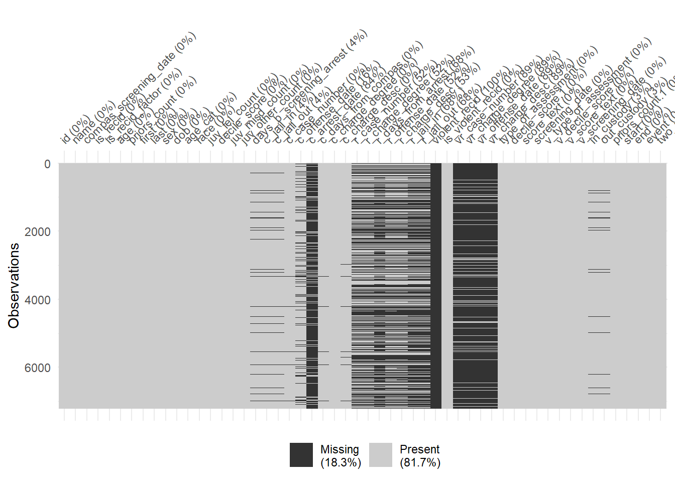
gg_miss_upset(data, nsets = 2, nintersects = 10) 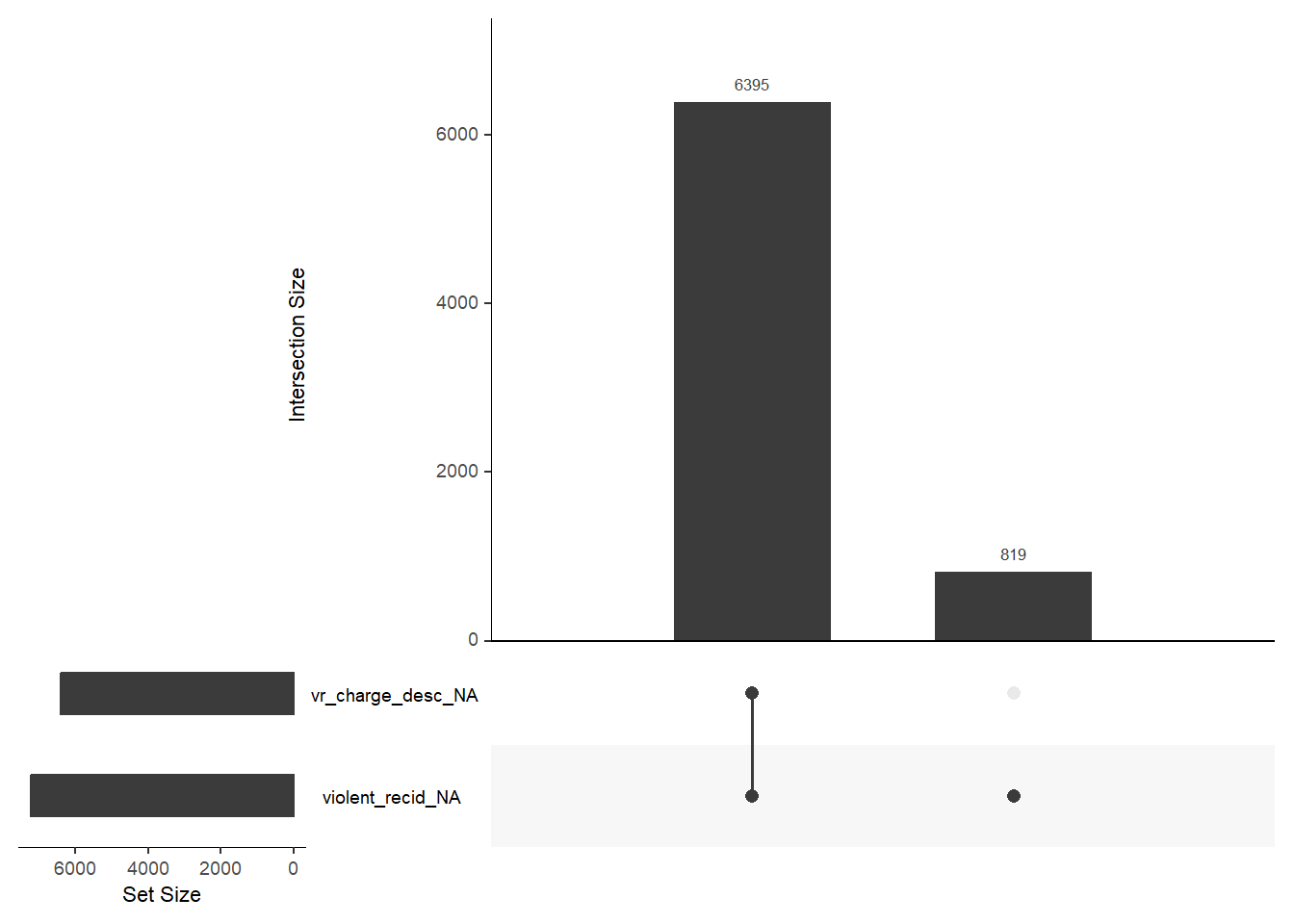
# Ideally, use higher number of nsets/nintersects
# with more screen space
4 Splitting the datasets
Below we split the data into training data and test data (Split 1). Then we further split (Split 2) the training data into an analysis dataset (sometimes also called training data) and an assessment dataset (often called validation set) (Kuhn and Johnson 2019). This is illustrated in Figure 1. We often call splits of the second kind folds. Below we have only one fold corresponding to “Resample 1” in Figure 1.

# Split the data into training and test data
  data_split <- initial_split(data, prop = 0.80)
  data_split # Inspect
<Training/Testing/Total>
<5771/1443/7214># Extract the two datasets
data_train <- training(data_split)
data_test <- testing(data_split) # Do not touch until the end!
# Further split the training data into analysis (training2) and assessment (validation) dataset
data_folds <- validation_split(data_train, prop = .80)
data_folds # Inspect# Validation Set Split (0.8/0.2)
# A tibble: 1 x 2
splits id
<list> <chr>
1 <split [4616/1155]> validation data_folds$splits # Inspect[[1]]
<Training/Validation/Total>
<4616/1155/5771> data_folds$splits[[1]] # Inspect<Training/Validation/Total>
<4616/1155/5771> # We have only 1 fold!
# Extract analysis ("training data 2") and assessment (validation) data
data_analysis <- analysis(data_folds$splits[[1]])
data_assessment <- assessment(data_folds$splits[[1]])
dim(data_analysis)[1] 4616 54 dim(data_assessment)[1] 1155 545 Building a predictive model
Dressel and Farid (2018) suggest that the COMPAS prediction (which apparently is based on 137 features) can be achieved with a simple linear classifier with only two features. Below we will try to replicate those results. Let’s fit the model now using our training data data_analysis:
fit <- glm(is_recid ~ age + priors_count,
family = binomial,
data = data_analysis)
#fit$coefficients
summary(fit)
Call:
glm(formula = is_recid ~ age + priors_count, family = binomial,
data = data_analysis)
Deviance Residuals:
Min 1Q Median 3Q Max
-2.9500 -1.0600 -0.5445 1.0949 2.2245
Coefficients:
Estimate Std. Error z value Pr(>|z|)
(Intercept) 1.078772 0.102684 10.51 <0.0000000000000002 ***
age -0.050219 0.003032 -16.56 <0.0000000000000002 ***
priors_count 0.173002 0.008905 19.43 <0.0000000000000002 ***
---
Signif. codes: 0 '***' 0.001 '**' 0.01 '*' 0.05 '.' 0.1 ' ' 1
(Dispersion parameter for binomial family taken to be 1)
Null deviance: 6392.1 on 4615 degrees of freedom
Residual deviance: 5667.4 on 4613 degrees of freedom
AIC: 5673.4
Number of Fisher Scoring iterations: 4An increase of 1 in the number of prior offences is associated with an increase of 0.17 in the log-odds of recidivism, all other things being equal.
An increase in age by one year corresponds to a decrease of -0.05 in the log-odds of recidivism.
- (If we’re being a bit silly and decide to extrapolate) according to the model, a newborn (in prison) with no prior offences would have a predicted probability of 0.75 of being re-arrested.
6 Predicting values (analysis data)
If no data set is supplied the predict() function computes probabilities for all units in data_analysis, i.e., the whole dataset (and all individuals) that we used to fit the model (see below). The probability is computed for each individual in our dataset, hence, we get a vector of the length of our dataset. And we can add those predicted probablity to the dataset (then we can check different individuals).
# Predict probability and add to data
data_analysis$y_hat <- predict(fit, type="response") # predict values for everyone and add to data
summary(data_analysis$y_hat) Min. 1st Qu. Median Mean 3rd Qu. Max.
0.04355 0.35929 0.48094 0.48050 0.57931 0.99621 Alternatively to predict() we can use the augment() function from the broom package.
broom::augment(fit)# A tibble: 4,616 x 9
is_recid age priors_count .fitted .resid .hat .sigma .cooksd .std.r~1
<dbl> <dbl> <dbl> <dbl> <dbl> <dbl> <dbl> <dbl> <dbl>
1 0 36 0 -0.729 -0.887 0.000402 1.11 0.0000648 -0.887
2 1 21 0 0.0242 1.17 0.000642 1.11 0.000209 1.17
3 1 28 7 0.884 0.832 0.000603 1.11 0.0000832 0.832
4 0 21 0 0.0242 -1.19 0.000642 1.11 0.000219 -1.19
5 0 25 2 0.169 -1.25 0.000397 1.11 0.000157 -1.25
6 1 26 0 -0.227 1.28 0.000460 1.11 0.000193 1.28
7 1 30 2 -0.0818 1.21 0.000282 1.11 0.000102 1.21
8 1 60 19 1.35 0.678 0.00368 1.11 0.000320 0.679
9 0 33 2 -0.232 -1.08 0.000264 1.11 0.0000697 -1.08
10 1 27 5 0.588 0.940 0.000439 1.11 0.0000814 0.940
# ... with 4,606 more rows, and abbreviated variable name 1: .std.residWe know that these values correspond to the probability of the recidivating/reoffending (rather than not), because the underlying dummy variable is 1 for reoffending (see use of contrasts() function in James et al. (2013, 158)).
We can also make predictions for particular hypothetical values of our explanatory variables/features.
Q: Does the predicted probability change as a consequence of age and prior offences?
data_predict = data.frame(age = c(30, 30, 50, 50),
priors_count = c(2, 4, 2, 4))
data_predict$y_hat <- predict(fit, newdata = data_predict, type = "response")
data_predict age priors_count y_hat
1 30 2 0.4795628
2 30 4 0.5656709
3 50 2 0.2523392
4 50 4 0.3229667We observe an increase of about 8% in the probability when changing the priors_count (number of prior offences) variable from 2 to 4 (keeping age at 30).
In the end we want to predict a binary outcome - NOT recidivate vs. recidivate. So let’s convert our predicted probabilities y_hat into a binary variable that classifies people into those that will recidivate or not. We call this variable y_hat_01 and it contains our model-based classification \(\hat{y}_{i}\) that we can compare to the actual behavior stored in is_recid.
We decide that we use a threshold of > 0.5 (of the probability) to classify people as (future) recidivators. Then we can create the variable y_hat_01 that contains our model-based classification \(\hat{y}_{i}\). Subsequently, we can compare it to the real outcome values \(y_{i}\) that are stored in the variable is_recid. See below.
data_analysis <- data_analysis %>%
mutate(y_hat_01 = if_else(y_hat >= 0.5, 1, 0))Let’s inspect the corresponding variables.
Q: What is what again?
head(data_analysis %>% select(is_recid, age,
priors_count, y_hat,
y_hat_01))# A tibble: 6 x 5
is_recid age priors_count y_hat y_hat_01
<dbl> <dbl> <dbl> <dbl> <dbl>
1 0 36 0 0.325 0
2 1 21 0 0.506 1
3 1 28 7 0.708 1
4 0 21 0 0.506 1
5 0 25 2 0.542 1
6 1 26 0 0.444 07 Accuracy: Analysis (training) data error rate
The training error rate is the error rate we make when making predictions in the training data (the data we use to built our predictive model).
Q: How would you interpret this table?
# Table y against predicted y
table(data_analysis$is_recid, data_analysis$y_hat_01)
0 1
0 1745 653
1 820 1398Answer
The diagonal elements of the confusion matrix indicate correct predictions, while the off-diagonals represent incorrect predictions.
Subsequently, we can calculate how many errors we made and the training error rate:
sum(data_analysis$is_recid!=data_analysis$y_hat_01) # number of errors[1] 1473- Q: How could we calculate the number of errors using the cross table above?
Answer
# Training error rate
# same as: sum(data_analysis$is_recid!=data_analysis$y_hat_01)/nrow(data_analysis)
mean(data_analysis$is_recid!=data_analysis$y_hat_01) # Error rate[1] 0.3191075sum(data_analysis$is_recid==data_analysis$y_hat_01) # Number of correct predictions[1] 3143# Correct classification rate
mean(data_analysis$is_recid==data_analysis$y_hat_01) # Correct rate[1] 0.6808925We can see that 0.32 of the individuals have been predicted wrongly by our classifier. 0.68 have been predicted correctly.
Q: Do you think this is high? What could be a benchmark?
8 Accuracy: Assessment (validation) data error rate
The assessment (validation) error rate is the error rate we make using our model in in the assessment (validation) dataset, i.e., the data that the model “has not seen yet” (but not the test dataset!).
We haven’t calculated this error rate yet, so let’s see how our model would perform in data_assessment that we held out. This error rate should be more realistic, since the model has not seen the data yet (cf. James et al. 2013, 158). Below we fit the model (again as above) on our analysis data, but then we do the predictions for the assessment (validation) dataset.
# Fit the model (again)
fit <- glm(is_recid ~ age + priors_count,
family = binomial,
data = data_analysis)
# Use model parameters to classify (predict) using the validation dataset
# and add to dataset
data_assessment$y_hat <- predict(fit, data_assessment ,type="response")Then we add the classification variable again, now in data_assessment, and calculate our error rates but now for the validation data:
# Add classification variable
data_assessment <- data_assessment %>%
mutate(y_hat_01 = if_else(y_hat >= 0.5, 1, 0))
mean(data_assessment$is_recid!=data_assessment$y_hat_01) # Error rate[1] 0.3082251mean(data_assessment$is_recid==data_assessment$y_hat_01) # Correct rate[1] 0.6917749We can see that the rates for the assessment (validation) dataset are very similar to those we obtained from our model for the training data.
Finally, we can also tabulate our predictions:
# Table y against predicted y
table(data_assessment$is_recid, data_assessment$y_hat_01)
0 1
0 450 155
1 201 3499 Accuracy: Test data error rate
Above we calculate the error rate for the assessment data. In this example we have one analysis dataset (often called the training dataset), one assessment dataset and one test dataset (cf. Figure 1). Above we calculated the error rate for the analysis and the assessment data. We would use the assessment data to try out different model specifications and evalute the predictive model.
The final test is done on the test dataset.
# Fit the model on the training data (again)
fit <- glm(is_recid ~ age + priors_count,
family = binomial,
data = data_analysis)
# Use model parameters to classify (predict)
# using the test dataset
# and add to test dataset
data_test$y_hat <- predict(fit, data_test, type="response")
# Add classification variable
data_test <- data_test %>%
mutate(y_hat_01 = if_else(y_hat >= 0.5, 1, 0))
# Calculate rates
mean(data_test$is_recid!=data_test$y_hat_01) # Error rate[1] 0.3250173mean(data_test$is_recid==data_test$y_hat_01) # Correct rate[1] 0.6749827# Table actual values against predictions
table(data_test$is_recid, data_test$y_hat_01)
0 1
0 544 196
1 273 430The error rate is slightly higher in the test dataset.
10 Using the list column workflow
Below we use the list column workflow to pursue the steps we did above for the analysis and the assessment data. Later we can use this strategy to do so across different folds/models
# Install packages
# install.packages(pacman)
pacman::p_load(tidyverse,
tidymodels)
# Load data
# data <-
# read_csv(sprintf("https://docs.google.com/uc?id=%s&export=download",
# "1plUxvMIoieEcCZXkBpj4Bxw1rDwa27tj"))
# Split the data into training and test data
data_split <- initial_split(data, prop = 0.80)
data_train <- training(data_split)
data_test <- testing(data_split) # Do not touch until the end!
data_folds <- validation_split(data_train, prop = .80)
# Use list column workflow to do different steps (1 model!)
# Assign to object to see content of single steps
data_folds %>%
# Create data_analysis and data_assessment
mutate(data_analysis = map(.x = splits, ~training(.x)),
data_assessment = map(.x = splits, ~testing(.x))) %>%
# Estimate model
mutate(model = map(data_analysis,
~glm(formula = is_recid ~ age + priors_count,
data = .x))) %>%
# Add model stats
mutate(model_stats = map(model, ~glance(.x))) %>%
# Analysis data: Extract y, add predictions y^,
# dichotomize predicted probability, caculate mean absolute error
mutate(y_analysis = map(data_analysis, ~.x$is_recid)) %>%
mutate(y_hat_analysis = map2(model, data_analysis,
~predict(.x, .y, type="response"))) %>%
mutate(y_hat_01_analysis = map(y_hat_analysis,
~if_else(.x >= 0.5, 1, 0))) %>%
mutate(mae_y_analysis = map2_dbl(y_analysis,
y_hat_01_analysis,
~Metrics::mae(actual = .x,
predicted = .y))) %>%
# Assessment data: Extract y, add predictions y^,
# dichotomize predicted probability, caculate mean absolute error
mutate(y_assessment = map(data_assessment, ~.x$is_recid)) %>%
mutate(y_hat_assessment = map2(model, data_assessment,
~predict(.x, .y, type="response"))) %>%
mutate(y_hat_01_assessment = map(y_hat_assessment,
~if_else(.x >= 0.5, 1, 0))) %>%
mutate(mae_y_assessment = map2_dbl(y_assessment,
y_hat_01_assessment,
~Metrics::mae(actual = .x,
predicted = .y))) %>%
# Select variables for display
select(splits, data_analysis, data_assessment,
mae_y_analysis, mae_y_assessment)# A tibble: 1 x 5
splits data_analysis data_assessment mae_y_anal~1 mae_y~2
<list> <list> <list> <dbl> <dbl>
1 <split [4616/1155]> <tibble [4,616 x 53]> <tibble> 0.323 0.318
# ... with abbreviated variable names 1: mae_y_analysis, 2: mae_y_assessmentHow would you interpret the results, i.e., mae_y_analysis and mae_y_assessment (size, difference, etc.)?
In principle, we could also try to integrate the data_split, data_train and data_test into the dataframe that contains the folds. However, since they are not really part of the model training, i.e., data_test is only used once at the very end, we usually do not want to carry them along. Above we split the training data only once (1 fold), later on we will extend this logic to further splits, models etc.
11 Exercise/homework: Building a predictive logistic model
- Start by loading the recidvism data into R and converting certain variables (you can use the code below).
- Follow the steps in the lab to split the dataset into training/test data (using
initial_split()) and then to split the training data into analysis/assessment data (usingvalidation_split()). - In our lab we used a logistic model to predict whether someone will recidiviate or not. So far we only used two variables/features to predict
is_recidnamelyageandpriors_count. Estimate this model usingdata_analysisand call the resultfit_1. Extend this model with three more predictors (race,sex,juv_fel_count), train the model and call the resultfit_2. - For both models add predictions
y_hat_1andy_hat_2todata_assessmentand dichotomize those predictions yieldingy_hat_1_01andy_hat_2_01.
- Compute the error rates in
data_assessmentof the two models with each other. Does the model with 5 predictors provide more accurate predictions? - Using your model
fit_2predict the probabilities of recidivism for three different ages (20, 40, 60 years). Keep that values of the other features at the following values:race = "African-American",sex = "Male"andjuv_fel_count = mean(data_analysis$juv_fel_count).
Hint: Maybe you can use the list column workflow to do some of the steps in the exercise.
# 1.
data <- read_csv(sprintf("https://docs.google.com/uc?id=%s&export=download",
"1plUxvMIoieEcCZXkBpj4Bxw1rDwa27tj"))
data <- data %>%
select(is_recid, age, priors_count, race, sex, juv_fel_count) %>%
mutate(sex = as_factor(sex),
race = as_factor(race))12 Exercise: What’s being predicted?
- Q: What do we predict using the techniques below? What is the input/what is the output? How could we use those ML models for research in our disciplines? (discuss 2!)
13 Exercise: Discussion
- Image recognition: Predict whether an image shows a sunsetSome examples
- Deepart: “Predict” what an image would look like if it was painted by…
- Speech recognition: Predict which (written) words someone just used
- Translation: Predict which English word/sentence corresponds to a German word/sentence (predict language!)
- Pose estimation (2018!): Predict body pose from image
- Deep fakes (2019): ?
- Text analysis/Natural language processing (NLP): Predict entities, sentiment, syntax, categories in text
14 All the code
# install.packages(pacman)
pacman::p_load(tidyverse,
tidymodels,
naniar)
data <- read_csv(sprintf("https://docs.google.com/uc?id=%s&export=download",
"1plUxvMIoieEcCZXkBpj4Bxw1rDwa27tj"))
data$is_recid_factor <- factor(data$is_recid,
levels = c(0,1),
labels = c("no", "yes"))
data <- data %>% select(id, name, compas_screening_date, is_recid,
is_recid_factor, age, priors_count, everything())
nrow(data)
ncol(data)
str(data) # Better use glimpse()
glimpse(data)
library(modelsummary)
datasummary_skim(data, type = "numeric", output = "html")
datasummary_skim(data, type = "categorical", output = "html")
table(data$race, useNA = "always")
table(data$is_recid, data$is_recid_factor)
table(data$decile_score)
vis_miss(data)
gg_miss_upset(data, nsets = 2, nintersects = 10)
# Ideally, use higher number of nsets/nintersects
# with more screen space
# Split the data into training and test data
data_split <- initial_split(data, prop = 0.80)
data_split # Inspect
# Extract the two datasets
  data_train <- training(data_split)
  data_test <- testing(data_split) # Do not touch until the end!

# Further split the training data into analysis (training2) and assessment (validation) dataset
  data_folds <- validation_split(data_train, prop = .80)
  data_folds # Inspect
data_folds$splits # Inspect
data_folds$splits[[1]] # Inspect
  # We have only 1 fold!

# Extract analysis ("training data 2") and assessment (validation) data
  data_analysis <- analysis(data_folds$splits[[1]])
  data_assessment <- assessment(data_folds$splits[[1]])
  dim(data_analysis)
dim(data_assessment)
fit <- glm(is_recid ~ age + priors_count,
           family = binomial,
           data = data_analysis)
#fit$coefficients
summary(fit)
x <- predict(fit,
newdata = data.frame(age = 0,
priors_count = 0), type = "response")
x <- round(x, 2)
# Predict probability and add to data
data_analysis$y_hat <- predict(fit, type="response") # predict values for everyone and add to data
summary(data_analysis$y_hat)
broom::augment(fit)
data_predict = data.frame(age = c(30, 30, 50, 50),
                 priors_count = c(2, 4, 2, 4))
data_predict$y_hat <- predict(fit, newdata = data_predict, type = "response")
data_predict
data_analysis <- data_analysis %>%
              mutate(y_hat_01 = if_else(y_hat >= 0.5, 1, 0))
head(data_analysis %>% select(is_recid, age,
                           priors_count, y_hat,
                           y_hat_01))
# Table y against predicted y
table(data_analysis$is_recid, data_analysis$y_hat_01)
sum(data_analysis$is_recid!=data_analysis$y_hat_01) # number of errors
# Training error rate
# same as: sum(data_analysis$is_recid!=data_analysis$y_hat_01)/nrow(data_analysis)
mean(data_analysis$is_recid!=data_analysis$y_hat_01) # Error rate
sum(data_analysis$is_recid==data_analysis$y_hat_01) # Number of correct predictions
# Correct classification rate
mean(data_analysis$is_recid==data_analysis$y_hat_01) # Correct rate
# Fit the model (again)
fit <- glm(is_recid ~ age + priors_count,
            family = binomial,
            data = data_analysis)

# Use model parameters to classify (predict) using the validation dataset
# and add to dataset
data_assessment$y_hat <- predict(fit, data_assessment ,type="response")
# Add classification variable
data_assessment <- data_assessment %>%
              mutate(y_hat_01 = if_else(y_hat >= 0.5, 1, 0))
mean(data_assessment$is_recid!=data_assessment$y_hat_01) # Error rate
mean(data_assessment$is_recid==data_assessment$y_hat_01) # Correct rate
# Table y against predicted y
table(data_assessment$is_recid, data_assessment$y_hat_01)
# Fit the model on the training data (again)
fit <- glm(is_recid ~ age + priors_count,
            family = binomial,
            data = data_analysis)

# Use model parameters to classify (predict)
# using the test dataset
# and add to test dataset
data_test$y_hat <- predict(fit, data_test, type="response")

# Add classification variable
data_test <- data_test %>%
              mutate(y_hat_01 = if_else(y_hat >= 0.5, 1, 0))

# Calculate rates
mean(data_test$is_recid!=data_test$y_hat_01) # Error rate
mean(data_test$is_recid==data_test$y_hat_01) # Correct rate
# Table actual values against predictions
table(data_test$is_recid, data_test$y_hat_01)
# Install packages
  # install.packages(pacman)
  pacman::p_load(tidyverse,
                 tidymodels)

# Load data
  # data <-
  # read_csv(sprintf("https://docs.google.com/uc?id=%s&export=download",
  # "1plUxvMIoieEcCZXkBpj4Bxw1rDwa27tj"))

# Split the data into training and test data
  data_split <- initial_split(data, prop = 0.80)
  data_train <- training(data_split)
  data_test <- testing(data_split) # Do not touch until the end!
  data_folds <- validation_split(data_train, prop = .80)

# Use list column workflow to do different steps (1 model!)
  # Assign to object to see content of single steps
  data_folds %>%

  # Create data_analysis and data_assessment
  mutate(data_analysis = map(.x = splits, ~training(.x)),
      data_assessment = map(.x = splits, ~testing(.x))) %>%

  # Estimate model
  mutate(model = map(data_analysis,
      ~glm(formula = is_recid ~ age + priors_count,
      data = .x))) %>%

  # Add model stats
  mutate(model_stats = map(model, ~glance(.x))) %>%

  # Analysis data: Extract y,  add predictions y^,
    # dichotomize predicted probability, caculate mean absolute error
  mutate(y_analysis = map(data_analysis, ~.x$is_recid)) %>%

  mutate(y_hat_analysis = map2(model, data_analysis,
      ~predict(.x, .y, type="response"))) %>%

  mutate(y_hat_01_analysis = map(y_hat_analysis,
      ~if_else(.x >= 0.5, 1, 0))) %>%

  mutate(mae_y_analysis = map2_dbl(y_analysis,
                                   y_hat_01_analysis,
                                   ~Metrics::mae(actual = .x,
                                                 predicted = .y))) %>%

  # Assessment data: Extract y,  add predictions y^,
    # dichotomize predicted probability, caculate mean absolute error
  mutate(y_assessment = map(data_assessment, ~.x$is_recid)) %>%

  mutate(y_hat_assessment = map2(model, data_assessment,
      ~predict(.x, .y, type="response"))) %>%

  mutate(y_hat_01_assessment = map(y_hat_assessment,
      ~if_else(.x >= 0.5, 1, 0))) %>%

  mutate(mae_y_assessment = map2_dbl(y_assessment,
                                     y_hat_01_assessment,
                                     ~Metrics::mae(actual = .x,
                                                   predicted = .y))) %>%

  # Select variables for display
    select(splits, data_analysis, data_assessment,
           mae_y_analysis, mae_y_assessment)
# 1.
data <- read_csv(sprintf("https://docs.google.com/uc?id=%s&export=download",
                         "1plUxvMIoieEcCZXkBpj4Bxw1rDwa27tj"))
data <- data %>%
  select(is_recid, age, priors_count, race, sex, juv_fel_count) %>%
  mutate(sex = as_factor(sex),
race = as_factor(race))References
Angwin, Julia, Jeff Larson, Lauren Kirchner, and Surya Mattu. 2016. “Machine Bias.” https://www.propublica.org/article/machine-bias-risk-assessments-in-criminal-sentencing.
Dressel, Julia, and Hany Farid. 2018. “The Accuracy, Fairness, and Limits of Predicting Recidivism.” Sci Adv 4 (1): eaao5580.
James, Gareth, Daniela Witten, Trevor Hastie, and Robert Tibshirani. 2013. An Introduction to Statistical Learning: With Applications in R. Springer Texts in Statistics. Springer.
Kuhn, Max, and Kjell Johnson. 2019. Feature Engineering and Selection: A Practical Approach for Predictive Models. CRC press (Taylor & Francis).
Lee, Claire S, Jeremy Du, and Michael Guerzhoy. 2020. “Auditing the COMPAS Recidivism Risk Assessment Tool: Predictive Modelling and Algorithmic Fairness in CS1.” In Proceedings of the 2020 ACM Conference on Innovation and Technology in Computer Science Education, 535–36. ITiCSE ’20. New York, NY, USA: Association for Computing Machinery.