| id | name | compas_screening_date | is_recid | is_recid_factor | age | priors_count |
|---|---|---|---|---|---|---|
| 1 | miguel hernandez | 2013-08-14 | 0 | no | 69 | 0 |
| 3 | kevon dixon | 2013-01-27 | 1 | yes | 34 | 0 |
| 4 | ed philo | 2013-04-14 | 1 | yes | 24 | 4 |
| 5 | marcu brown | 2013-01-13 | 0 | no | 23 | 1 |
| 6 | bouthy pierrelouis | 2013-03-26 | 0 | no | 43 | 2 |
| 7 | marsha miles | 2013-11-30 | 0 | no | 44 | 0 |
| 8 | edward riddle | 2014-02-19 | 1 | yes | 41 | 14 |
| 9 | steven stewart | 2013-08-30 | 0 | no | 43 | 3 |
| 10 | elizabeth thieme | 2014-03-16 | 0 | no | 39 | 0 |
| 13 | bo bradac | 2013-11-04 | 1 | yes | 21 | 1 |
Binary classification (logistic model)
Learning outcomes/objective: Learn…
- …and repeat logic underlying logistic model.
- …that there is a (joint-)distribution underlying and model.
- …how to assess accuracy (logistic regression).
- …concepts (training dataset etc.) using a “simple example”.
1 Predicting Recidvism (1): The data
2 Predicting Recidvism (2): The Logistic Model
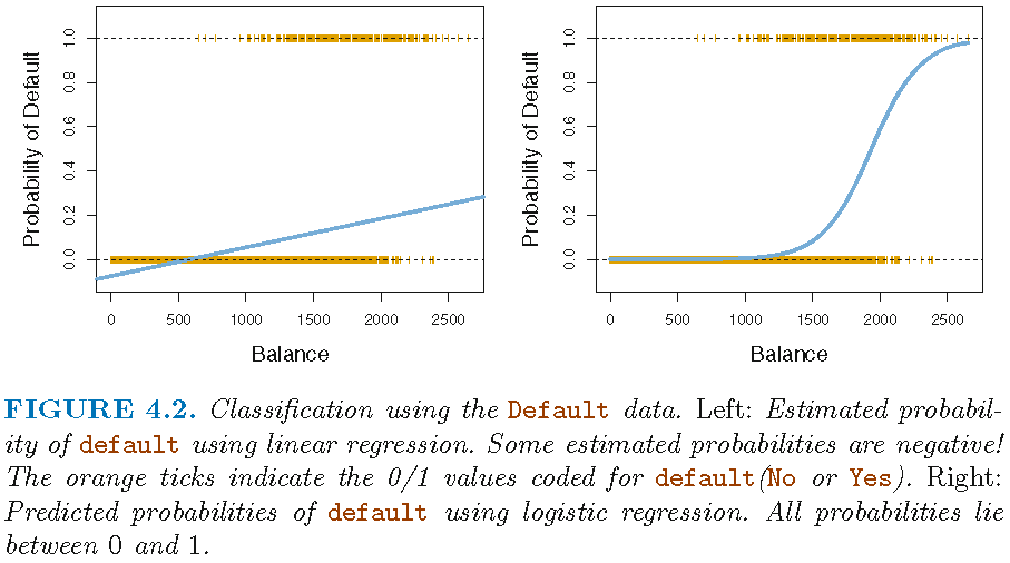
- Predicting recidivsm (0/1): How should we model the relationship between \(Pr(Y=1|X)=p(X)\) and \(X\)?
- See Figure 1 below
- Use either linear probability model or logistic regression
- Linear probability model: \(p(X)=\beta_{0}+\beta_{1}X\)
- Linear predictions of our outcome (probabilities), can be out of [0,1] range
- Logistic regression: \(p(X)=\frac{e^{\beta_{0}+\beta_{1}X}}{1+e^{\beta_{0}+\beta_{1}X}}\)
- …force them into range using logistic function
- odds: \(\frac{p(X)}{1-p(X)}=e^{\beta_{0}+\beta_{1}X}\) (range: \([0,\infty]\), the higher, the higher probability of recidivism/default)
- log-odds/logit: \(log\left(\frac{p(X)}{1-p(X)}\right) = \beta_{0}+\beta_{1}X\) (James et al. 2013, 132)
- …take logarithm on both sides.
- Increasing X by one unit, increases the log odds by \(\beta_{1}\) (usually output/interpretation in R)
- Estimation of \(\beta_{0}\) and \(\beta_{1}\) usually relies on maximum likelihood
- Source: James et al. (2013, chaps. 4.3.1, 4.3.2, 4.3.4)
3 Predicting Recidvism (3)
- Logistic regression (LR) models the probability that \(Y\) belongs to a particular category (0 or 1)
- Rather than modeling response \(Y\) directly
- COMPAS data: Model probability to recidivate (reoffend)
- Outcome \(y\): Recidivism
is_recid(0,1,0,0,1,1,...) - Various predictors \(x's\)
- age =
age - prior offenses =
priors_count
- age =
- Outcome \(y\): Recidivism
- Use LR to obtain predicted values \(\hat{y}\)
- As probabilities predicted values will range between 0 and 1
- Depend on input/features (e.g., age, prior offences)
- Convert predicted values (probabilities) to a binary variable
- e.g., predict individuals will recidivate (
is_recid = Yes) if Pr(is_recid=Yes|age) > 0.5 - Here we call this variable
y_hat_01
- e.g., predict individuals will recidivate (
- Source: James et al. (2013, chap. 4.3)
4 Predicting Recidvism (4): Model estimation
- Estimate model in R: glm(y ~ x1 + x2, family = binomial, data = data_train)
fit <- glm(as.factor(is_recid) ~ age + priors_count,
           family = binomial,
           data = data_train)
cat(paste(capture.output(summary(fit))[11:14], collapse="\n"))
Estimate Std. Error z value Pr(>|z|)
(Intercept) 1.101001 0.097597 11.28 <0.0000000000000002 ***
age -0.049831 0.002861 -17.42 <0.0000000000000002 ***
priors_count 0.159982 0.008236 19.43 <0.0000000000000002 ***- R output shows log odds: e.g., a one-unit increase in
ageis associated with an increase in the log odds ofis_recidby-0.05units - Difficult to interpret.. much easier to use predicted probabilities
5 Predicting Recidvism (5): Use model to predict
predict(): Predict values in R (oraugment())- Once coefficients have been estimated, it is a simple matter to compute the probability of outcome for values of our predictors (James et al. 2013, 134)
predict(fit, newdata = NULL, type = "response"): Predict probability for each unit- Use argument
type="response"to output probabilities of form \(P(Y=1|X)\) (as opposed to other information such as the logit)
predict(fit, newdata = data_predict, type = "response"): Predict probability setting values for particular Xs (contained indata_predict)
data_predict = data.frame(age = c(20, 20, 40, 40),
                          priors_count = c(0, 2, 0, 2))
data_predict$y_hat <- predict(fit, newdata = data_predict, type = "response")
data_predict
age priors_count y_hat
1 20 0 0.5260711
2 20 2 0.6045219
3 40 0 0.2906473
4 40 2 0.3607111- Q: How would you interpret these values?
- Source: James et al. (2013, chaps. 4.3.3, 4.6.2)
6 Predicting Recidvism (6)
- Background story by ProPublica: Machine Bias
- Methodology: How We Analyzed the COMPAS Recidivism Algorithm
- Replication and extension by Dressel and Farid (2018): The Accuracy, Fairness, and Limits of Predicting Recidivism
- Abstract: “Algorithms for predicting recidivism are commonly used to assess a criminal defendant’s likelihood of committing a crime. […] used in pretrial, parole, and sentencing decisions. […] We show, however, that the widely used commercial risk assessment software COMPAS is no more accurate or fair than predictions made by people with little or no criminal justice expertise. In addition, despite COMPAS’s collection of 137 features, the same accuracy can be achieved with a simple linear classifier with only two features.”
- Very nice lab by Lee, Du, and Guerzhoy (2020): Auditing the COMPAS Score: Predictive Modeling and Algorithmic Fairness
- We will work with the corresponding data and use it to grasp various concepts underlying statistical/machine learning
References
Dressel, Julia, and Hany Farid. 2018. “The Accuracy, Fairness, and Limits of Predicting Recidivism.” Sci Adv 4 (1): eaao5580.
James, Gareth, Daniela Witten, Trevor Hastie, and Robert Tibshirani. 2013. An Introduction to Statistical Learning: With Applications in R. Springer Texts in Statistics. Springer.
Lee, Claire S, Jeremy Du, and Michael Guerzhoy. 2020. “Auditing the COMPAS Recidivism Risk Assessment Tool: Predictive Modelling and Algorithmic Fairness in CS1.” In Proceedings of the 2020 ACM Conference on Innovation and Technology in Computer Science Education, 535–36. ITiCSE ’20. New York, NY, USA: Association for Computing Machinery.