Feature selection & regularization

Learning outcomes/objective: Learn…

• …about model regularization/feature selection (focus on ridge regression and lasso).
• …how to implement ridge regression and lasso in R with tidymodels.
• …what a tuning parameter can be used for (\(\lambda\) in ridge regression/lasso)

Sources: James et al. (2013, Ch. 6), ISLR tidymodels labs by Emil Hvitfeldt

1 Fundstücke/findings

• Reid Hoffmann on ChatGPT

2 Concepts

• Feature selection: also known as variable selection, attribute selection or variable subset selection, is the process of selecting a subset of relevant features (variables, predictors) for use in model construction (Wikipedia)
• Regularization: In ML either choice of the model or modifications to the algorithm

3 Why using alternatives to least squares?

• Why use another fitting procedure instead of least squares? (James et al. 2013, Ch. 6)
  • Alternative fitting procedures can yield better prediction accuracy and model interpretability
• Prediction Accuracy: Provided that the true relationship between the response and the predictors is approximately linear, the least squares estimates will have low bias
  • If \(n \gg p\) (much larger) least squares estimates have low bias but if not possibility of overfitting
  • By constraining or shrinking the estimated coefficients, we can often substantially reduce the variance at the cost of negligible increase in bias (James et al. 2013, 204)
• Model Interpretability: Often the case that some/many of the variables used in a multiple regression model are in fact not associated with the response/outcome
  • Including such irrelevant variables leads to unnecessary complexity in resulting model
  • Idea: remove these variables (set corresponding coefficient estimates to 0) to obtain a model that is more easily interpreted
  • There are various methods to do so automatically

4 Methods for feature/variables selection

• Subset selection: involves identifying subset of the \(p\) predictors that we believe to be related to the response
  • Strategy: Fit a model using least squares on the reduced set of variables
  • e.g., best subset selection (James et al. 2013, Ch. 6.1.1), forward/backward stepwise selection (relying on model fit) (James et al. 2013, Ch. 6.1.2)
  • Tidymodels: “It’s not a huge priority since other methods (e.g. regularization) are uniformly superior methods to feature selection.” (Source)
• Shrinkage: involves fitting a model involving all \(p\) predictors but shrink coefficients to zero relative to the least squares estimates
  • This shrinkage (also known as regularization) has the effect of reducing variance
  • Depending on what type of shrinkage is performed, some coefficients may be estimated to be exactly zero,i.e., shrinkage methods can perform variable selection
  • e.g., ridge regression (James et al. 2013, Ch. 6.2.1), the lasso (James et al. 2013, Ch. 6.2.2)
• Dimension Reduction: involves projecting the \(p\) predictors into a M-dimensional subspace, where \(M<p\).
  • This is achieved by computing \(M\) different linear combinations (or projections) of the variables.
  • Then these \(M\) projections are used as predictors to fit a linear regression model by least squares
  • e.g., principal components regression (James et al. 2013, Ch. 6.3.1), partial least squares (James et al. 2013, Ch. 6.3.2)

5 High dimensional data

• “Most traditional statistical techniques for regression and classification are intended for the low-dimensional setting in which \(n\), the number of observations, is much greater than \(p\), the number of features” (James et al. 2013, 238)
• “Data sets containing more features than observations are often referred to as high-dimensional. Classical approaches such as least squares linear regression are not appropriate in this setting.” (James et al. 2013, 239)
• “It turns out that many of the methods seen in this chapter for fitting less flexible least squares models, such as forward stepwise selection, ridge regression, the lasso, and principal components regression, are particularly useful for performing regression in the high-dimensional setting. Essentially, these approaches avoid overfitting by using a less flexible fitting approach than least squares.” (James et al. 2013, 239)

6 Ridge regression (RR) (1)

• Least squares (LS) estimator: least squares fitting procedure estimates \(\beta_{0}, \beta_{1}, ..., \beta_{p}\) using the values that minimize RSS
• Ridge regression (RR): seeks coefficient estimates that fit data well (minimize RSS) + shrinkage penalty
  • See formula (6.5) in (James et al. 2013, 215)
• shrinkage penalty \(\lambda \sum_{j=1}^{p}\beta_{j}^{2}\) is small when \(\beta_{0}, \beta_{1}, ..., \beta_{p}\) close to zero
  • penality has effect of shrinking the estimates \(\beta_{j}\) to zero
  • Tuning parameter \(\lambda\) serves to control the relative impact of these two terms (RSS and shrinking penalty) on the regression coefficient estimates
    • When \(\lambda = 0\) the penalty term has no effect and ridge regression will produce least squares estimates
    • As \(\lambda \rightarrow \infty\), impact of the shrinkage penalty grows, and the ridge regression coefficient estimates will approach zero
  • Penality is only applied to coefficients not the intercept
• Ridge regression will produce a different set of coefficient estimates \(\hat{\beta}_{\lambda}^{R}\) for each \(\lambda\)
  • Hyperparameter tuning: fit many models with different \(\lambda\)s to find the model the performs “best”

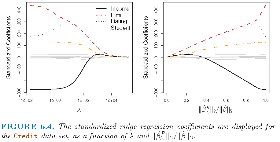
7 Ridge regression (RR) (2): Visualization

• Figure 1 displays regression coefficient estimates for the Credit data (James et al. 2013, Ch. 6.2)
  • Left-hand panel: each curve corresponds to the ridge regression coefficient estimate for one of the ten variables, plotted as a function of \(\lambda\)
    • to the left \(\lambda\) is essentially zero, so ridge coefficient estimates are the same as the usual least squares estimates
    • as \(\lambda\) increases, ridge coefficient estimates shrink towards zero
    • when \(\lambda\) is extremely large, all of the ridge coefficient estimates are basically zero = null model
• Occasionally coefficients can increase as \(\lambda\) increases (cf. predictor “Rating”)
• While standard LS coefficient estimates are scale equivalent, RR coefficients are not
  • Best to apply ridge regression after standardizing the predictors (resulting in SD = 1 for all predictors and final fit independent of predictor scales)

Figure 1: Source: James et al. (2013), Ch. 6.2, Figure 6.4

8 Ridge regression (RR) (3): Why?

• Why Does Ridge Regression (RR) Improve Over Least Squares (LS)?

• Advantage rooted in the bias-variance trade-off
  • As \(\lambda\) increases, flexibility of ridge regression fit decreases, leading to decreased variance but increased bias
    • Q: What was variance and bias again in the context of ML? (see here)
• In situations where relationship between response (outcome) and predictors is close to linear, LS estimates will have low bias but may have high variance
  • \(\rightarrow\) small change in the training data can cause a large change in the LS coefficient estimates
  • In particular, when number of variables \(p\) is almost as large as the number of observations \(n\) (cf. James et al. 2013, fig. 6.5), LS estimates will be extremely variable
  • If \(p>n\), then LS estimates do not even have a unique solution, whereas RR can still perform well
• Summary: RR works best in situations where the LS estimates have high variance

9 The Lasso

• Ridge regression (RR) has one obvious disadvantage
  • Unlike subset selection methods (best subset, forward stepwise, and backward stepwise selection) that select models that involve a variable subset, RR will include all \(p\) predictors in final model
  • Penalty \(\lambda \sum_{j=1}^{p}\beta_{j}^{2}\) will shrink all coefficients towards zero, but no set them exactly to 0 (unless \(\lambda = \infty\))
  • No problem for accuracy, but challenging for model interpretation when \(p\) is large
• Lasso (least absolute shrinkage and selection operator)
  • As in RR lasso shrinks the coefficient estimates towards zero but additionally…
  • …its penality has effect of forcing some of the coefficient estimates to be exactly equal to zero when tuning parameter \(\lambda\) is sufficiently large (cf. James et al. 2013, Eq. 6.7, p.219)
  • LASSO performs variable selection leading to easier interpretation, i.e., yields sparse models
  • As in RR selecting good value of \(\lambda\) is critical

10 Comparing the Lasso and Ridge Regression

• Advantage of Lasso: produces simpler and more interpret able models involving subset of predictors
• However, which method leads to better prediction accuracy?
  • Neither ridge regression nor lasso universally dominates the other
  • Lasso works better when few predictors have significant coefficients, others have small/zero coefficients
  • Ridge regression performs better with many predictors of roughly equal size
  • Cross-validation helps determine the better approach for a specific data set
  • Both methods can reduce variance at the cost of slight bias increase, improving prediction accuracy

11 Lab: Ridge Regression & Lasso

We’ll use the ESS data that we have used in the previous lab. The variables were not named so well, so we have to rely on the codebook to understand their meaning. You can find it here or on the website of the ESS.

• stflife: measures life satisfaction (How satisfied with life as a whole).
• uempla: measures unemployment (Doing last 7 days: unemployed, actively looking for job).
• uempli: measures life satisfaction (Doing last 7 days: unemployed, not actively looking for job).
• eisced: measures education (Highest level of education, ES - ISCED).
• cntry: measures a respondent’s country of origin (here held constant for France).
• etc.

We first import the data into R:

library(tidyverse)
library(tidymodels)

# Build and evaluate model without resampling
data <- read_csv(sprintf("https://docs.google.com/uc?id=%s&export=download",
                         "1azBdvM9-tDVQhADml_qlXjhpX72uHdWx"))

11.1 Renaming and recoding

Below we recode missings and also rename some of our variables (for easier interpretation later on):

data <- data  %>%
    filter(cntry=="FR") %>% # filter french respondents 
 # Recode missings
 mutate(ppltrst = if_else(ppltrst %in% c(55, 66, 77, 88, 99), NA, ppltrst),
        eisced = if_else(eisced %in% c(55, 66, 77, 88, 99), NA, eisced),
        stflife = if_else(stflife %in% c(55, 66, 77, 88, 99), NA, stflife)) %>%
 # Rename variables
 rename(country = cntry,
        unemployed_active = uempla,
        unemployed = uempli,
        trust = ppltrst,
        lifesatisfaction = stflife,
        education = eisced,
        age = agea,
        religion = rlgdnm,
        children_number = chldo12) %>% # we add this variable
  mutate(religion = factor(recode(religion, # Recode and factor
    "1" = "Roman Catholic",
    "2" = "Protestant",
    "3" = "Eastern Orthodox",
    "4" = "Other Christian denomination",
    "5" = "Jewish",
    "6" = "Islam",
    "7" = "Eastern religions",
    "8" = "Other Non-Christian religions",
    .default = NA_character_))) %>%
  select(lifesatisfaction, 
        unemployed_active,
        unemployed,
        trust,
        lifesatisfaction,
        education,
        age,
        religion,
        health,
        children_number)  %>%
  filter(!is.na(lifesatisfaction))
kable(head(data))

lifesatisfaction	unemployed_active	unemployed	trust	education	age	religion	health	children_number
10	0	0	5	4	23	Roman Catholic	2	0
7	0	0	7	6	32	NA	2	0
7	0	0	5	4	25	NA	2	0
5	0	0	7	1	74	Roman Catholic	4	0
7	0	0	4	4	39	Roman Catholic	2	0
10	0	0	3	3	59	NA	3	2

11.2 Split the data

Below we split the data and create resampled partitions with vfold_cv() stored in an object called data_folds. Hence, we have the original data_train and data_test but also already resamples of data_train in data_folds.

# Split the data into training and test data
  data_split <- initial_split(data, prop = 0.80)
  data_split # Inspect

<Training/Testing/Total>
<1576/395/1971>

# Extract the two datasets
  data_train <- training(data_split)
  data_test <- testing(data_split) # Do not touch until the end!

# Create resampled partitions
  set.seed(345)
  data_folds <- vfold_cv(data_train, v = 10) # V-fold/k-fold cross-validation
  data_folds # data_folds now contains several resamples of our training data  

#  10-fold cross-validation 
# A tibble: 10 x 2
   splits             id    
   <list>             <chr> 
 1 <split [1418/158]> Fold01
 2 <split [1418/158]> Fold02
 3 <split [1418/158]> Fold03
 4 <split [1418/158]> Fold04
 5 <split [1418/158]> Fold05
 6 <split [1418/158]> Fold06
 7 <split [1419/157]> Fold07
 8 <split [1419/157]> Fold08
 9 <split [1419/157]> Fold09
10 <split [1419/157]> Fold10

  # You can also try loo_cv(data_train) instead

11.3 Simple ridge regression (all in one)

Below we provide a quick example of a ridge regression (beware: we did not standardize the predictors since this can easily be done in a recipe).

• Arguments of glmnet linear_reg()
  • mixture = 0: to specify a ridge model
    • mixture = 0 specifies only ridge regularization
    • mixture = 1 specifies only lasso regularization
    • Setting mixture to a value between 0 and 1 lets us use both
  • penalty = 0: Penality we need to set when using glmnet engine (for now 0)

# Define and fit the mdoel
  ridge_fit <- linear_reg(mixture = 0, penalty = 0) %>%
  set_mode("regression") %>%
  set_engine("glmnet") %>%
  fit(formula = lifesatisfaction ~ .,
                   data = data_train)
  
# Extract coefficients
  tidy(ridge_fit)

# A tibble: 13 x 3
   term                                   estimate penalty
   <chr>                                     <dbl>   <dbl>
 1 (Intercept)                            5.42           0
 2 unemployed_active                     -0.177          0
 3 unemployed                            -1.18           0
 4 trust                                  0.205          0
 5 education                              0.114          0
 6 age                                   -0.000833       0
 7 religionEastern religions             -0.406          0
 8 religionIslam                          0.244          0
 9 religionJewish                        -0.543          0
10 religionOther Christian denomination  -1.02           0
11 religionOther Non-Christian religions  0.0907         0
12 religionProtestant                    -0.294          0
13 religionRoman Catholic                 0.434          0

# Extract coefficients for particular penalty values
  tidy(ridge_fit, penalty = 350)

# A tibble: 13 x 3
   term                                     estimate penalty
   <chr>                                       <dbl>   <dbl>
 1 (Intercept)                            7.12           350
 2 unemployed_active                     -0.00224        350
 3 unemployed                            -0.00728        350
 4 trust                                  0.00138        350
 5 education                              0.000972       350
 6 age                                   -0.00000715     350
 7 religionEastern religions             -0.00309        350
 8 religionIslam                         -0.000981       350
 9 religionJewish                        -0.00545        350
10 religionOther Christian denomination  -0.00861        350
11 religionOther Non-Christian religions  0.00158        350
12 religionProtestant                    -0.00359        350
13 religionRoman Catholic                 0.00261        350

# Visualize how magnitude of coefficients are being 
# regularized towards zero as penalty goes up
  ridge_fit %>%
  autoplot()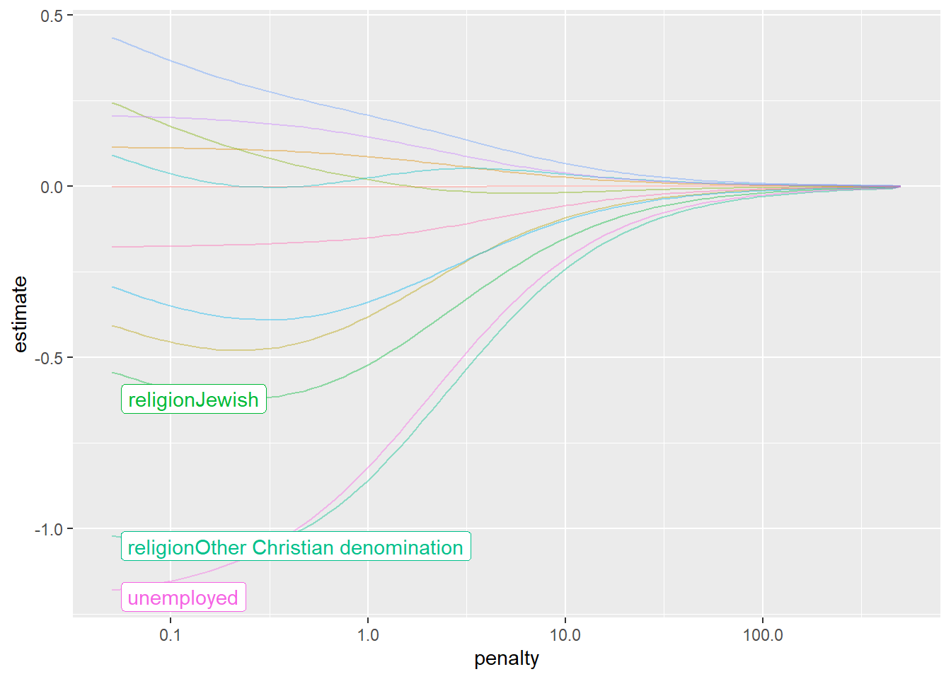

# Use fitted model to predict values  
  predict(ridge_fit, new_data = data_test)

# A tibble: 395 x 1
   .pred
   <dbl>
 1  7.10
 2  6.70
 3  7.62
 4  6.76
 5  7.59
 6 NA   
 7 NA   
 8  7.09
 9  6.26
10  7.92
# ... with 385 more rows

11.4 Finding/tuning the best penalty value

Above we saw that we can fit a ridge regression model and get predictions for different penality values. However, to maximize accuracy we woudl like to identify the “best” penalty value. Here we use hyperparameter tuning. Below we keep it simple and try different values for \(\lambda\) using grid search and evenly spaced parameter values. For tuning we also rely on resampling.

Above we already created our 10-fold cross-validation dataset stored in data_folds. We proceed to define our recipe.

Q: What are the different step functions doing? (e.g., ?step_zv)

# Define recipe
ridge_recipe <- 
  recipe(formula = lifesatisfaction ~ ., data = data_train) %>% 
  step_naomit(all_predictors()) %>%
  step_novel(all_nominal_predictors()) %>% # necessary?
  step_dummy(all_nominal_predictors()) %>% 
  step_zv(all_predictors()) %>% 
  step_normalize(all_predictors())

Then we specify the model. It’s similar to previous labs only that we set penalty = tune() to tell tune_grid() that the penalty parameter should be tuned.

# Define model
ridge_model <- 
  linear_reg(penalty = tune(), mixture = 0) %>% 
  set_mode("regression") %>% 
  set_engine("glmnet")

Then we define a workflow called ridge_workflow that includes our recipe and model specification.

ridge_workflow <- workflow() %>% 
  add_recipe(ridge_recipe) %>% 
  add_model(ridge_model)

And we use grid_regular() to create a grid of evenly spaced parameter values. In it we use the penalty() function (dials package) to denote the parameter and set the range of the grid. Computation is fast so we can choose a fine-grained grid with 50 levels.

penalty_grid <- grid_regular(penalty(range = c(-5, 5)), levels = 50)
penalty_grid

# A tibble: 50 x 1
     penalty
       <dbl>
 1 0.00001  
 2 0.0000160
 3 0.0000256
 4 0.0000409
 5 0.0000655
 6 0.000105 
 7 0.000168 
 8 0.000268 
 9 0.000429 
10 0.000687 
# ... with 40 more rows

Then we can fit all our models using the resamples in data_folds using the tune_grid function.

tune_result <- tune_grid(
  ridge_workflow,
  resamples = data_folds, 
  grid = penalty_grid
)

tune_result

# Tuning results
# 10-fold cross-validation 
# A tibble: 10 x 4
   splits             id     .metrics           .notes          
   <list>             <chr>  <list>             <list>          
 1 <split [1418/158]> Fold01 <tibble [100 x 5]> <tibble [2 x 3]>
 2 <split [1418/158]> Fold02 <tibble [100 x 5]> <tibble [2 x 3]>
 3 <split [1418/158]> Fold03 <tibble [100 x 5]> <tibble [2 x 3]>
 4 <split [1418/158]> Fold04 <tibble [100 x 5]> <tibble [2 x 3]>
 5 <split [1418/158]> Fold05 <tibble [100 x 5]> <tibble [2 x 3]>
 6 <split [1418/158]> Fold06 <tibble [100 x 5]> <tibble [2 x 3]>
 7 <split [1419/157]> Fold07 <tibble [100 x 5]> <tibble [2 x 3]>
 8 <split [1419/157]> Fold08 <tibble [100 x 5]> <tibble [2 x 3]>
 9 <split [1419/157]> Fold09 <tibble [100 x 5]> <tibble [2 x 3]>
10 <split [1419/157]> Fold10 <tibble [100 x 5]> <tibble [2 x 3]>

There were issues with some computations:

  - Warning(s) x10: There are new levels in a factor: NAThere were 12 warnings in `dp...   - Warning(s) x10: There are new levels in a factor: NAThere were 12 warnings in `dp...

Run `show_notes(.Last.tune.result)` for more information.

And use autoplot to visualize the results.

Q: What does the graph show?

autoplot(tune_result)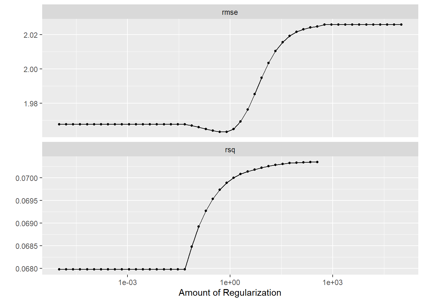

Yes, it visualizes how the performance metrics are impacted by our parameter choice of the regularization parameter, i.e, penalty \(\lambda\). We can also collected the metrics:

collect_metrics(tune_result)

# A tibble: 100 x 7
     penalty .metric .estimator   mean     n std_err .config              
       <dbl> <chr>   <chr>       <dbl> <int>   <dbl> <chr>                
 1 0.00001   rmse    standard   1.97      10  0.0617 Preprocessor1_Model01
 2 0.00001   rsq     standard   0.0680    10  0.0140 Preprocessor1_Model01
 3 0.0000160 rmse    standard   1.97      10  0.0617 Preprocessor1_Model02
 4 0.0000160 rsq     standard   0.0680    10  0.0140 Preprocessor1_Model02
 5 0.0000256 rmse    standard   1.97      10  0.0617 Preprocessor1_Model03
 6 0.0000256 rsq     standard   0.0680    10  0.0140 Preprocessor1_Model03
 7 0.0000409 rmse    standard   1.97      10  0.0617 Preprocessor1_Model04
 8 0.0000409 rsq     standard   0.0680    10  0.0140 Preprocessor1_Model04
 9 0.0000655 rmse    standard   1.97      10  0.0617 Preprocessor1_Model05
10 0.0000655 rsq     standard   0.0680    10  0.0140 Preprocessor1_Model05
# ... with 90 more rows

Afterwards select_best() can be used to extract the best parameter value.

best_penalty <- select_best(tune_result, metric = "rsq")
best_penalty

# A tibble: 1 x 2
  penalty .config              
    <dbl> <chr>                
1    356. Preprocessor1_Model38

11.5 Finalize workflow, assess accuracy and extract predicted values

Finally, we can update our workflow with finalize_workflow() and set the penalty to best_penalty that we stored above, and fit the model on our training data.

# Define final workflow
ridge_final <- finalize_workflow(ridge_workflow, best_penalty)
ridge_final

== Workflow ====================================================================
Preprocessor: Recipe
Model: linear_reg()

-- Preprocessor ----------------------------------------------------------------
5 Recipe Steps

* step_naomit()
* step_novel()
* step_dummy()
* step_zv()
* step_normalize()

-- Model -----------------------------------------------------------------------
Linear Regression Model Specification (regression)

Main Arguments:
  penalty = 355.648030622313
  mixture = 0

Computational engine: glmnet 

# Fit the model
ridge_final_fit <- fit(ridge_final, data = data_train)

We then evaluate the accuracy of this model (that is based on the training data) using the test data data_test. We use augment() to obtain the predictions:

# Use fitted model to predict values  
  augment(ridge_final_fit, new_data = data_test)

# A tibble: 395 x 8
   lifesatisfaction unemployed_active unempl~1 trust educa~2   age relig~3 .pred
              <dbl>             <dbl>    <dbl> <dbl>   <dbl> <dbl> <fct>   <dbl>
 1                7                 0        0     4       4    39 Roman ~  7.13
 2                9                 0        0     2       4    18 Roman ~  7.13
 3                7                 0        0     5       7    63 Roman ~  7.13
 4                3                 0        0     3       3    62 Roman ~  7.13
 5                6                 0        0     7       3    53 Roman ~  7.13
 6                8                 0        0     4       7    42 <NA>    NA   
 7                8                 0        0     3       4    31 <NA>    NA   
 8                8                 0        0     5       2    17 Roman ~  7.13
 9                8                 0        0     0       4    54 Roman ~  7.12
10                8                 0        0     8       4    33 Roman ~  7.13
# ... with 385 more rows, and abbreviated variable names 1: unemployed,
#   2: education, 3: religion

And can directly pipe the result into functions such as rsq(), rmse() and mae() to obtain the corresponding measures of accuracy.

augment(ridge_final_fit, new_data = data_test) %>%
  rsq(truth = lifesatisfaction, estimate = .pred)

# A tibble: 1 x 3
  .metric .estimator .estimate
  <chr>   <chr>          <dbl>
1 rsq     standard       0.111

augment(ridge_final_fit, new_data = data_test) %>%
  rmse(truth = lifesatisfaction, estimate = .pred)

# A tibble: 1 x 3
  .metric .estimator .estimate
  <chr>   <chr>          <dbl>
1 rmse    standard        2.11

augment(ridge_final_fit, new_data = data_test) %>%
    mae(truth = lifesatisfaction, estimate = .pred)

# A tibble: 1 x 3
  .metric .estimator .estimate
  <chr>   <chr>          <dbl>
1 mae     standard        1.61

12 Lab: Lasso

Below the same steps but now using Lasso.

# Define the recipe
lasso_recipe <- 
  recipe(formula = lifesatisfaction ~ ., data = data_train) %>% 
  step_naomit(all_predictors()) %>%
  step_novel(all_nominal_predictors()) %>% 
  step_dummy(all_nominal_predictors()) %>% 
  step_zv(all_predictors()) %>% 
  step_normalize(all_predictors())

# Specify the model
lasso_model <- 
  linear_reg(penalty = tune(), mixture = 1) %>% 
  set_mode("regression") %>% 
  set_engine("glmnet") 

# Define the workflow
lasso_workflow <- workflow() %>% 
  add_recipe(lasso_recipe) %>% 
  add_model(lasso_model)

# Define the penalty grid
penalty_grid <- grid_regular(penalty(range = c(-2, 2)), levels = 50)

# Tune the model and visualize
  tune_result <- tune_grid(
    lasso_workflow,
    resamples = data_folds, 
    grid = penalty_grid
  )
  
  autoplot(tune_result)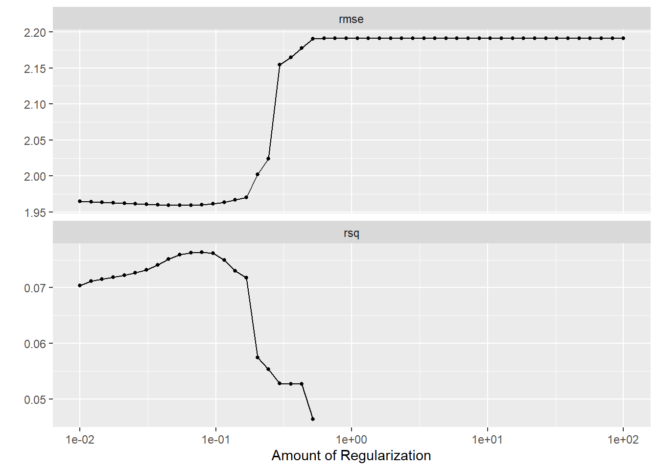

# Select best penalty
best_penalty <- select_best(tune_result, metric = "rsq")


# Finalize workflow and fit model
lasso_final <- finalize_workflow(lasso_workflow, best_penalty)

lasso_final_fit <- fit(lasso_final, data = data_train)


# Check accuracy in training data
  augment(lasso_final_fit, new_data = data_train) %>%
    mae(truth = lifesatisfaction, estimate = .pred)

# A tibble: 1 x 3
  .metric .estimator .estimate
  <chr>   <chr>          <dbl>
1 mae     standard        1.49

# Add predicted values to test data
augment(lasso_final_fit, new_data = data_test)

# A tibble: 395 x 8
   lifesatisfaction unemployed_active unempl~1 trust educa~2   age relig~3 .pred
              <dbl>             <dbl>    <dbl> <dbl>   <dbl> <dbl> <fct>   <dbl>
 1                7                 0        0     4       4    39 Roman ~  7.05
 2                9                 0        0     2       4    18 Roman ~  6.68
 3                7                 0        0     5       7    63 Roman ~  7.47
 4                3                 0        0     3       3    62 Roman ~  6.78
 5                6                 0        0     7       3    53 Roman ~  7.51
 6                8                 0        0     4       7    42 <NA>    NA   
 7                8                 0        0     3       4    31 <NA>    NA   
 8                8                 0        0     5       2    17 Roman ~  7.06
 9                8                 0        0     0       4    54 Roman ~  6.32
10                8                 0        0     8       4    33 Roman ~  7.77
# ... with 385 more rows, and abbreviated variable names 1: unemployed,
#   2: education, 3: religion

# Assess accuracy (RSQ)
augment(lasso_final_fit, new_data = data_test) %>%
  rsq(truth = lifesatisfaction, estimate = .pred)

# A tibble: 1 x 3
  .metric .estimator .estimate
  <chr>   <chr>          <dbl>
1 rsq     standard       0.120

# Assess accuracy (MAE)
augment(lasso_final_fit, new_data = data_test) %>%
  mae(truth = lifesatisfaction, estimate = .pred)

# A tibble: 1 x 3
  .metric .estimator .estimate
  <chr>   <chr>          <dbl>
1 mae     standard        1.52

13 Homework

1. Use the data from above (European Social Survey (ESS)) (below the code to get you started) and start by recoding/renaming variables so that you have at least 30 features/predictors that you can use (see codebook). Obviously, it would be good to include features that might be connected to life satisfaction.
2. Then built three models stored in workflow1 for a simple linear predictive model, workflow2 for a ridge regression and workflow3 for a lasso regression. You may need different recipes.
3. Train these three workflows and evaluate their accuracy using resampling.
4. Finally, evaluate their accuracy in the test dataset. The idea is to have at least one workflow that beats the accuracy metrics (focus on MAE) in the lab above.

# HOMEWORK: Build and evaluate model without resampling
data <- read_csv(sprintf("https://docs.google.com/uc?id=%s&export=download",
                         "1azBdvM9-tDVQhADml_qlXjhpX72uHdWx"))
data <- data  %>%
    filter(cntry=="FR") %>% # filter french respondents 
 # Recode missings
 mutate(ppltrst = if_else(ppltrst %in% c(55, 66, 77, 88, 99), NA, ppltrst),
        eisced = if_else(eisced %in% c(55, 66, 77, 88, 99), NA, eisced),
        stflife = if_else(stflife %in% c(55, 66, 77, 88, 99), NA, stflife)) %>%
 # Rename variables
 rename(country = cntry,
        unemployed_active = uempla,
        unemployed = uempli,
        trust = ppltrst,
        lifesatisfaction = stflife,
        education = eisced,
        age = agea)

14 All the code

# namer::unname_chunks("03_01_predictive_models.qmd")
# namer::name_chunks("03_01_predictive_models.qmd")
options(scipen=99999)

#| echo: false
library(tidyverse)
library(lemon)
library(knitr)
library(kableExtra)
library(dplyr)
library(plotly)
library(randomNames)
library(stargazer)
library(tidyverse)
library(tidymodels)

# Build and evaluate model without resampling
data <- read_csv(sprintf("https://docs.google.com/uc?id=%s&export=download",
                         "1azBdvM9-tDVQhADml_qlXjhpX72uHdWx"))
data <- data  %>%
    filter(cntry=="FR") %>% # filter french respondents 
 # Recode missings
 mutate(ppltrst = if_else(ppltrst %in% c(55, 66, 77, 88, 99), NA, ppltrst),
        eisced = if_else(eisced %in% c(55, 66, 77, 88, 99), NA, eisced),
        stflife = if_else(stflife %in% c(55, 66, 77, 88, 99), NA, stflife)) %>%
 # Rename variables
 rename(country = cntry,
        unemployed_active = uempla,
        unemployed = uempli,
        trust = ppltrst,
        lifesatisfaction = stflife,
        education = eisced,
        age = agea,
        religion = rlgdnm,
        children_number = chldo12) %>% # we add this variable
  mutate(religion = factor(recode(religion, # Recode and factor
    "1" = "Roman Catholic",
    "2" = "Protestant",
    "3" = "Eastern Orthodox",
    "4" = "Other Christian denomination",
    "5" = "Jewish",
    "6" = "Islam",
    "7" = "Eastern religions",
    "8" = "Other Non-Christian religions",
    .default = NA_character_))) %>%
  select(lifesatisfaction, 
        unemployed_active,
        unemployed,
        trust,
        lifesatisfaction,
        education,
        age,
        religion,
        health,
        children_number)  %>%
  filter(!is.na(lifesatisfaction))
kable(head(data))
# Split the data into training and test data
  data_split <- initial_split(data, prop = 0.80)
  data_split # Inspect

# Extract the two datasets
  data_train <- training(data_split)
  data_test <- testing(data_split) # Do not touch until the end!

# Create resampled partitions
  set.seed(345)
  data_folds <- vfold_cv(data_train, v = 10) # V-fold/k-fold cross-validation
  data_folds # data_folds now contains several resamples of our training data  
  # You can also try loo_cv(data_train) instead
# Define and fit the mdoel
  ridge_fit <- linear_reg(mixture = 0, penalty = 0) %>%
  set_mode("regression") %>%
  set_engine("glmnet") %>%
  fit(formula = lifesatisfaction ~ .,
                   data = data_train)
  
# Extract coefficients
  tidy(ridge_fit)
  
# Extract coefficients for particular penalty values
  tidy(ridge_fit, penalty = 350)
  
# Visualize how magnitude of coefficients are being 
# regularized towards zero as penalty goes up
  ridge_fit %>%
  autoplot()
  
# Use fitted model to predict values  
  predict(ridge_fit, new_data = data_test)
  
# Define recipe
ridge_recipe <- 
  recipe(formula = lifesatisfaction ~ ., data = data_train) %>% 
  step_naomit(all_predictors()) %>%
  step_novel(all_nominal_predictors()) %>% # necessary?
  step_dummy(all_nominal_predictors()) %>% 
  step_zv(all_predictors()) %>% 
  step_normalize(all_predictors())
# Define model
ridge_model <- 
  linear_reg(penalty = tune(), mixture = 0) %>% 
  set_mode("regression") %>% 
  set_engine("glmnet")
ridge_workflow <- workflow() %>% 
  add_recipe(ridge_recipe) %>% 
  add_model(ridge_model)
penalty_grid <- grid_regular(penalty(range = c(-5, 5)), levels = 50)
penalty_grid
tune_result <- tune_grid(
  ridge_workflow,
  resamples = data_folds, 
  grid = penalty_grid
)

tune_result

autoplot(tune_result)

collect_metrics(tune_result)
best_penalty <- select_best(tune_result, metric = "rsq")
best_penalty
# Define final workflow
ridge_final <- finalize_workflow(ridge_workflow, best_penalty)
ridge_final

# Fit the model
ridge_final_fit <- fit(ridge_final, data = data_train)
augment(ridge_final_fit, new_data = data_test) %>%
  rsq(truth = lifesatisfaction, estimate = .pred)

augment(ridge_final_fit, new_data = data_test) %>%
  rmse(truth = lifesatisfaction, estimate = .pred)
  
augment(ridge_final_fit, new_data = data_test) %>%
    mae(truth = lifesatisfaction, estimate = .pred)
# Use fitted model to predict values  
  augment(ridge_final_fit, new_data = data_test)
# Define the recipe
lasso_recipe <- 
  recipe(formula = lifesatisfaction ~ ., data = data_train) %>% 
  step_naomit(all_predictors()) %>%
  step_novel(all_nominal_predictors()) %>% 
  step_dummy(all_nominal_predictors()) %>% 
  step_zv(all_predictors()) %>% 
  step_normalize(all_predictors())

# Specify the model
lasso_model <- 
  linear_reg(penalty = tune(), mixture = 1) %>% 
  set_mode("regression") %>% 
  set_engine("glmnet") 

# Define the workflow
lasso_workflow <- workflow() %>% 
  add_recipe(lasso_recipe) %>% 
  add_model(lasso_model)

# Define the penalty grid
penalty_grid <- grid_regular(penalty(range = c(-2, 2)), levels = 50)

# Tune the model and visualize
  tune_result <- tune_grid(
    lasso_workflow,
    resamples = data_folds, 
    grid = penalty_grid
  )
  
  autoplot(tune_result)

# Select best penalty
best_penalty <- select_best(tune_result, metric = "rsq")


# Finalize workflow and fit model
lasso_final <- finalize_workflow(lasso_workflow, best_penalty)

lasso_final_fit <- fit(lasso_final, data = data_train)


# Check accuracy in training data
  augment(lasso_final_fit, new_data = data_train) %>%
    mae(truth = lifesatisfaction, estimate = .pred)


# Add predicted values to test data
augment(lasso_final_fit, new_data = data_test)


# Assess accuracy (RSQ)
augment(lasso_final_fit, new_data = data_test) %>%
  rsq(truth = lifesatisfaction, estimate = .pred)

# Assess accuracy (MAE)
augment(lasso_final_fit, new_data = data_test) %>%
  mae(truth = lifesatisfaction, estimate = .pred)


# HOMEWORK: Build and evaluate model without resampling
data <- read_csv(sprintf("https://docs.google.com/uc?id=%s&export=download",
                         "1azBdvM9-tDVQhADml_qlXjhpX72uHdWx"))
data <- data  %>%
    filter(cntry=="FR") %>% # filter french respondents 
 # Recode missings
 mutate(ppltrst = if_else(ppltrst %in% c(55, 66, 77, 88, 99), NA, ppltrst),
        eisced = if_else(eisced %in% c(55, 66, 77, 88, 99), NA, eisced),
        stflife = if_else(stflife %in% c(55, 66, 77, 88, 99), NA, stflife)) %>%
 # Rename variables
 rename(country = cntry,
        unemployed_active = uempla,
        unemployed = uempli,
        trust = ppltrst,
        lifesatisfaction = stflife,
        education = eisced,
        age = agea)

References

James, Gareth, Daniela Witten, Trevor Hastie, and Robert Tibshirani. 2013. An Introduction to Statistical Learning: With Applications in R. Springer Texts in Statistics. Springer.