# install.packages(pacman)
pacman::p_load(tidyverse,
               tidymodels,
               naniar,
               knitr,
kableExtra)Lab: Linear regression for prediction
Learning outcomes/objective: Learn…
- …how we can use the linear regression model as a ML model within R.
Sources: #TidyTuesday and tidymodels
1 Lab: ML using a linear model
Below we’ll use the European Social Survey (ESS) [Round 10 - 2020. Democracy, Digital social contacts] to illustrate how to use linear models for machine learning. The ESS contains different outcomes amenable to both classification and regression as well as a lot of variables that could be used as features (~580 variables). And we’ll focus on the french survey respondents.
The variables were named not so well, so we have to rely on the codebook to understand their meaning. You can find it here or on the website of the ESS.
stflife: measures life satisfaction (How satisfied with life as a whole).uempla: measures unemployment (Doing last 7 days: unemployed, actively looking for job).uempli: measures life satisfaction (Doing last 7 days: unemployed, not actively looking for job).eisced: measures education (Highest level of education, ES - ISCED).cntry: measures a respondent’s country of origin (here held constant for France).- etc.
We first import the data into R:
# Build and evaluate model without resampling
data <- read_csv(sprintf("https://docs.google.com/uc?id=%s&export=download",
                         "1azBdvM9-tDVQhADml_qlXjhpX72uHdWx"))
1.1 Renaming and recoding
The variables in the dataset contain various missings that we need to recode (because they are not stored as NA). We can explore them using the table function:
table(data$stflife, useNA = "always")
   0    1    2    3    4    5    6    7    8    9   10   77   88   99 <NA>
406 225 625 1128 1320 3659 3294 6227 7980 4591 3553 126 178 39 0 table(data$ppltrst, useNA = "always")
   0    1    2    3    4    5    6    7    8    9   10   77   88   99 <NA>
2607 1298 2398 3475 3240 6097 3648 4831 3792 1107  747   29   68   14    0
Hence, we recode those missings and also rename some of our variables (for easier interpretation later on):
data <- data  %>%
    filter(cntry=="FR") %>% # filter french respondents
 # Recode missings
 mutate(ppltrst = if_else(ppltrst %in% c(55, 66, 77, 88, 99), NA, ppltrst),
        eisced = if_else(eisced %in% c(55, 66, 77, 88, 99), NA, eisced),
        stflife = if_else(stflife %in% c(55, 66, 77, 88, 99), NA, stflife)) %>%
 # Rename variables
 rename(country = cntry,
        unemployed_active = uempla,
        unemployed = uempli,
        trust = ppltrst,
        lifesatisfaction = stflife,
        education = eisced,
        age = agea)
Q: Why did we filter respondents first (filter(cntry=="FR"))?
1.2 Inspecting the dataset
First we should make sure to really explore/unterstand our data. How many observations are there? How many different variables (features) are there? What is the scale of the outcome (here we focus on life satisfaction)? What are the averages etc.? What kind of units are in your dataset?
nrow(data)[1] 1977ncol(data)[1] 586# str(data)
# glimpse(data)Also always inspect summary statistics for both numeric and categorical variables to get a better understanding of the data. Often such summary statistics will also reveal (coding) errors in the data. Here we take a subset because the are too many variables (>250).
Q: Does anything strike you as interesting the two tables below?
library(modelsummary)
data_summary <- data %>%
select(lifesatisfaction, unemployed_active, unemployed, education, age)
datasummary_skim(data_summary, type = "numeric", output = "html")| Unique (#) | Missing (%) | Mean | SD | Min | Median | Max | ||
|---|---|---|---|---|---|---|---|---|
| lifesatisfaction | 12 | 0 | 7.0 | 2.2 | 0.0 | 7.0 | 10.0 |  |
| unemployed_active | 2 | 0 | 0.0 | 0.2 | 0.0 | 0.0 | 1.0 |  |
| unemployed | 2 | 0 | 0.0 | 0.1 | 0.0 | 0.0 | 1.0 |  |
| education | 8 | 1 | 4.1 | 1.9 | 1.0 | 4.0 | 7.0 |  |
| age | 76 | 0 | 51.0 | 41.4 | 16.0 | 50.0 | 999.0 |  |
# datasummary_skim(data_summary, type = "categorical", output = "html")The table() function is also useful to get an overview of variables. Use the argument useNA = "always" to display potential missings.
table(data$lifesatisfaction, useNA = "always")
0 1 2 3 4 5 6 7 8 9 10 <NA>
38 15 45 56 82 196 195 361 516 233 234 6 table(data$education, data$lifesatisfaction)
0 1 2 3 4 5 6 7 8 9 10
1 9 5 8 6 6 28 25 30 36 14 28
2 3 1 3 3 12 19 18 37 35 18 25
3 17 5 13 19 27 63 54 59 107 44 45
4 4 3 12 12 20 31 37 69 110 49 48
5 1 1 3 6 8 28 25 56 76 36 31
6 1 0 1 4 1 10 13 36 46 16 15
7 3 0 4 5 8 17 22 73 101 55 42round(prop.table(table(data$Education, data$Lifesatisfaction)),2)<0 x 0 matrix>Finally, there are some helpful functions to explore missing data included in the naniar package. Here we do so for a subset of variables. Can you decode those graphs? What do they show? (for publications the design would need to be improved)
vis_miss(data %>%
select(lifesatisfaction,
unemployed_active,
unemployed,
education,
age))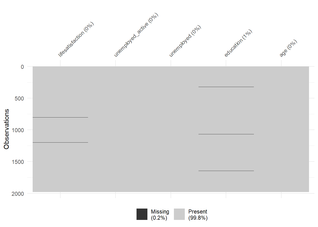
gg_miss_upset(data %>%
select(lifesatisfaction,
unemployed_active,
unemployed,
education,
age), nsets = 10, nintersects = 10) 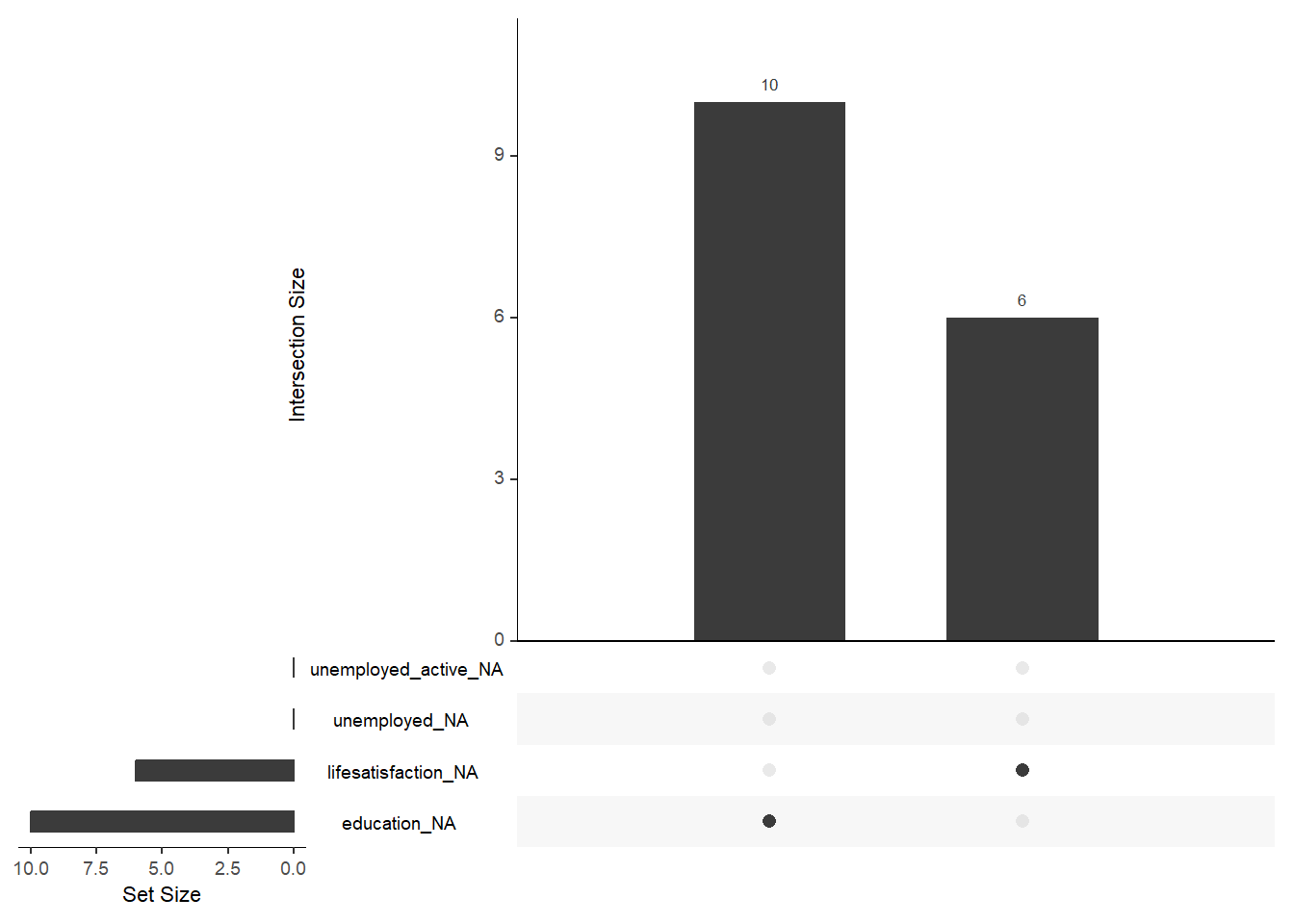
1.3 Building and evaluating a first predictive linear model
1.4 Split the data
Below we split the data and create resampled partitions with vfold_cv().
# Split the data into training and test data
data_split <- initial_split(data, prop = 0.80)
data_split # Inspect<Training/Testing/Total>
<1581/396/1977># Extract the two datasets
data_train <- training(data_split)
data_test <- testing(data_split) # Do not touch until the end!
# Create resampled partitions
set.seed(345)
data_folds <- vfold_cv(data_train, v = 10) # V-fold/k-fold cross-validation
data_folds # data_folds now contains several resamples of our training data # 10-fold cross-validation
# A tibble: 10 x 2
splits id
<list> <chr>
1 <split [1422/159]> Fold01
2 <split [1423/158]> Fold02
3 <split [1423/158]> Fold03
4 <split [1423/158]> Fold04
5 <split [1423/158]> Fold05
6 <split [1423/158]> Fold06
7 <split [1423/158]> Fold07
8 <split [1423/158]> Fold08
9 <split [1423/158]> Fold09
10 <split [1423/158]> Fold10 # You can also try loo_cv(data_train) instead1.5 Define model, recipe and workflow
Then we define our model and define a first workflow.
# Define the model
linear_mod <-
linear_reg() %>% # linear model
set_engine("lm") %>%
set_mode("regression")
# Create workflow
wflow1 <-
workflow() %>%
add_model(linear_mod) %>%
add_formula(lifesatisfaction ~ unemployed_active + age)1.6 Fit/train the model/workflow
Then we use this workflow to fit/train our model using the fit_resamples() function which provides more robust metrics to assess our model (across folds).
# Use workflow to fit the to train the model
# There is no need in specifying data_analysis/data_assessment as
# the functions understand the corresponding parts
fit_rs1 <-
wflow1 %>%
fit_resamples(resamples = data_folds)
fit_rs1# Resampling results
# 10-fold cross-validation
# A tibble: 10 x 4
splits id .metrics .notes
<list> <chr> <list> <list>
1 <split [1422/159]> Fold01 <tibble [2 x 4]> <tibble [0 x 3]>
2 <split [1423/158]> Fold02 <tibble [2 x 4]> <tibble [0 x 3]>
3 <split [1423/158]> Fold03 <tibble [2 x 4]> <tibble [0 x 3]>
4 <split [1423/158]> Fold04 <tibble [2 x 4]> <tibble [0 x 3]>
5 <split [1423/158]> Fold05 <tibble [2 x 4]> <tibble [0 x 3]>
6 <split [1423/158]> Fold06 <tibble [2 x 4]> <tibble [0 x 3]>
7 <split [1423/158]> Fold07 <tibble [2 x 4]> <tibble [0 x 3]>
8 <split [1423/158]> Fold08 <tibble [2 x 4]> <tibble [0 x 3]>
9 <split [1423/158]> Fold09 <tibble [2 x 4]> <tibble [0 x 3]>
10 <split [1423/158]> Fold10 <tibble [2 x 4]> <tibble [0 x 3]>Q: Do you remember how we can extract the first two rows of .metrics?
1.7 Evaluate the model/workflow
Then we use collect_metrics() to evaluate our models averaging across our resamples, accounting for the natural variability across different analysis datasets that we could possibly use to built the model.
# Collect metrics across resamples
metrics1 <- collect_metrics(fit_rs1)
metrics1# A tibble: 2 x 6
.metric .estimator mean n std_err .config
<chr> <chr> <dbl> <int> <dbl> <chr>
1 rmse standard 2.22 10 0.0689 Preprocessor1_Model1
2 rsq standard 0.0140 10 0.00613 Preprocessor1_Model1The average (across folds) RMSE (Root Mean Squared Error) is 2.22 and the average R-squared (rsq) is 0.01.
1.8 Compare with another workflow
Using workflows we can easily compare two a linear models with one more predictor namely education simply piping the different steps together. Below we create a second workflow as comparison.
# Create a second workflow with one more variable
wflow2 <-
workflow() %>%
add_model(linear_mod) %>%
add_formula(lifesatisfaction ~ unemployed_active + age + education)
# Fit the workflow and directly assess metrics
wflow2 %>%
fit_resamples(resamples = data_folds) %>%
collect_metrics()# A tibble: 2 x 6
.metric .estimator mean n std_err .config
<chr> <chr> <dbl> <int> <dbl> <chr>
1 rmse standard 2.15 10 0.0417 Preprocessor1_Model1
2 rsq standard 0.0334 10 0.00686 Preprocessor1_Model1Q: How does the accuracy change when adding the predictor education?
1.9 Use workflow for final model/prediction
Finally, when we are happy with one of the models/workflows (after our assessment using resampling) we can fit the model/workflow to data_train (not using any resampling) and use it to predict the outcome in our data_test to calculate the accuracy. Below we use wflow2.1
# Fit the model/workflow to data_train
fit2 <-
wflow2 %>%
fit(data = data_train)
fit2== Workflow [trained] ==========================================================
Preprocessor: Formula
Model: linear_reg()
-- Preprocessor ----------------------------------------------------------------
lifesatisfaction ~ unemployed_active + age + education
-- Model -----------------------------------------------------------------------
Call:
stats::lm(formula = ..y ~ ., data = data)
Coefficients:
(Intercept) unemployed_active age education
6.271827 -0.189836 -0.001725 0.209567 # Extract coefficients for inspection
fit2 %>%
extract_fit_parsnip() %>%
tidy()# A tibble: 4 x 5
term estimate std.error statistic p.value
<chr> <dbl> <dbl> <dbl> <dbl>
1 (Intercept) 6.27 0.148 42.3 5.81e-261
2 unemployed_active -0.190 0.303 -0.627 5.31e- 1
3 age -0.00173 0.00119 -1.45 1.49e- 1
4 education 0.210 0.0293 7.15 1.30e- 12# Calculate accuracy for training data
augment(fit2, data_train) %>%
select(lifesatisfaction, unemployed_active, age, education, .pred) %>%
rmse(truth = lifesatisfaction, estimate = .pred)# A tibble: 1 x 3
.metric .estimator .estimate
<chr> <chr> <dbl>
1 rmse standard 2.14# Augment data_test with predictions and subset variables
#fit2 %>% predict(new_data = data_test) # Alternative
data_test <- augment(fit2, data_test) %>%
select(lifesatisfaction, unemployed_active, age, education, .pred)
data_test# A tibble: 396 x 5
lifesatisfaction unemployed_active age education .pred
<dbl> <dbl> <dbl> <dbl> <dbl>
1 7 0 32 6 7.47
2 9 0 51 2 6.60
3 7 0 31 7 7.69
4 10 0 38 7 7.67
5 9 0 45 7 7.66
6 5 0 62 3 6.79
7 8 0 44 7 7.66
8 9 0 38 3 6.83
9 8 0 53 3 6.81
10 10 0 31 5 7.27
# ... with 386 more rows# Calculate accuracy
data_test %>%
rmse(truth = lifesatisfaction, estimate = .pred)# A tibble: 1 x 3
.metric .estimator .estimate
<chr> <chr> <dbl>
1 rmse standard 2.33The accuracy is slightly worse for the test data as compared to the training data.
2 Homework/Exercise
Use the data from above (below the code to get you started) and built a predictive linear model using a workflow that provides a better accuracy for predicting life satisfaction then the two models outlines in the lab (lifesatisfaction ~ unemployed_active + age vs. lifesatisfaction ~ unemployed_active + age + education). You can choose as any and as many predictors you want from the European Social Survey (ESS) [Round 10 - 2020. Democracy, Digital social contacts] and the codebook should help you in the selection. Remember to recode the respective variables if necessary.
# HOMEWORK: Build and evaluate model without resampling
data <- read_csv(sprintf("https://docs.google.com/uc?id=%s&export=download",
"1azBdvM9-tDVQhADml_qlXjhpX72uHdWx"))
data <- data %>%
filter(cntry=="FR") %>% # filter french respondents
# Recode missings
mutate(ppltrst = if_else(ppltrst %in% c(55, 66, 77, 88, 99), NA, ppltrst),
eisced = if_else(eisced %in% c(55, 66, 77, 88, 99), NA, eisced),
stflife = if_else(stflife %in% c(55, 66, 77, 88, 99), NA, stflife)) %>%
# Rename variables
rename(country = cntry,
unemployed_active = uempla,
unemployed = uempli,
trust = ppltrst,
lifesatisfaction = stflife,
education = eisced,
age = agea)3 All the code
# install.packages(pacman)
pacman::p_load(tidyverse,
tidymodels,
naniar,
knitr,
kableExtra)
# Build and evaluate model without resampling
data <- read_csv(sprintf("https://docs.google.com/uc?id=%s&export=download",
"1azBdvM9-tDVQhADml_qlXjhpX72uHdWx"))
table(data$stflife, useNA = "always")
table(data$ppltrst, useNA = "always")
data <- data %>%
filter(cntry=="FR") %>% # filter french respondents
# Recode missings
mutate(ppltrst = if_else(ppltrst %in% c(55, 66, 77, 88, 99), NA, ppltrst),
eisced = if_else(eisced %in% c(55, 66, 77, 88, 99), NA, eisced),
stflife = if_else(stflife %in% c(55, 66, 77, 88, 99), NA, stflife)) %>%
# Rename variables
rename(country = cntry,
unemployed_active = uempla,
unemployed = uempli,
trust = ppltrst,
lifesatisfaction = stflife,
education = eisced,
age = agea)
nrow(data)
ncol(data)
# str(data)
# glimpse(data)
library(modelsummary)
data_summary <- data %>%
  select(lifesatisfaction, unemployed_active, unemployed, education, age)
datasummary_skim(data_summary, type = "numeric", output = "html")
# datasummary_skim(data_summary, type = "categorical", output = "html")
table(data$lifesatisfaction, useNA = "always")
table(data$education, data$lifesatisfaction)
round(prop.table(table(data$Education, data$Lifesatisfaction)),2)
vis_miss(data %>%
                select(lifesatisfaction,
                       unemployed_active,
                       unemployed,
                       education,
                       age))
gg_miss_upset(data %>%
                select(lifesatisfaction,
                       unemployed_active,
                       unemployed,
                       education,
                       age), nsets = 10, nintersects = 10)
# Split the data into training and test data
  data_split <- initial_split(data, prop = 0.80)
  data_split # Inspect
# Extract the two datasets
  data_train <- training(data_split)
  data_test <- testing(data_split) # Do not touch until the end!

# Create resampled partitions
  set.seed(345)
  data_folds <- vfold_cv(data_train, v = 10) # V-fold/k-fold cross-validation
  data_folds # data_folds now contains several resamples of our training data
# You can also try loo_cv(data_train) instead
# Define the model
  linear_mod <-
  linear_reg() %>% # linear model
  set_engine("lm") %>%
  set_mode("regression")

# Create workflow
  wflow1 <-
  workflow() %>%
  add_model(linear_mod) %>%
  add_formula(lifesatisfaction ~ unemployed_active + age)
# Use workflow to fit the to train the model
  # There is no need in specifying data_analysis/data_assessment as
  # the functions understand the corresponding parts
  fit_rs1 <-
  wflow1 %>%
  fit_resamples(resamples = data_folds)
  fit_rs1
# Collect metrics across resamples
  metrics1 <- collect_metrics(fit_rs1)
  metrics1
# Create a second workflow with one more variable
  wflow2 <-
  workflow() %>%
  add_model(linear_mod) %>%
  add_formula(lifesatisfaction ~ unemployed_active + age + education)

# Fit the workflow and directly assess metrics
  wflow2 %>%
  fit_resamples(resamples = data_folds) %>%
  collect_metrics()
# HOMEWORK: Build and evaluate model without resampling
data <- read_csv(sprintf("https://docs.google.com/uc?id=%s&export=download",
                         "1azBdvM9-tDVQhADml_qlXjhpX72uHdWx"))
data <- data  %>%
    filter(cntry=="FR") %>% # filter french respondents
 # Recode missings
 mutate(ppltrst = if_else(ppltrst %in% c(55, 66, 77, 88, 99), NA, ppltrst),
        eisced = if_else(eisced %in% c(55, 66, 77, 88, 99), NA, eisced),
        stflife = if_else(stflife %in% c(55, 66, 77, 88, 99), NA, stflife)) %>%
 # Rename variables
 rename(country = cntry,
        unemployed_active = uempla,
        unemployed = uempli,
        trust = ppltrst,
        lifesatisfaction = stflife,
        education = eisced,
age = agea)Footnotes
There is current research on model averaging prediction by k-fold cross-validation.↩︎