8.4 Nonlinear Effects on Test Scores of the Student-Teacher Ratio
In this section we will discuss three specific questions about the relationship between test scores and the student-teacher ratio:
Does the effect on test scores of decreasing the student-teacher ratio depend on the fraction of English learners when we control for economic idiosyncrasies of the different districts?
Does this effect depend on the the student-teacher ratio?
How strong is the effect of decreasing the student-teacher ratio (by two students per teacher) if we take into account economic characteristics and nonlinearities?
Too answer these questions we consider a total of seven models, some of which are nonlinear regression specifications of the types that have been discussed before. As measures for the students’ economic backgrounds, we additionally consider the regressors \(lunch\) and \(\ln(income)\). We use the logarithm of \(income\) because the analysis in Chapter 8.2 showed that the nonlinear relationship between \(income\) and \(TestScores\) is approximately logarithmic. We do not include expenditure per pupil (\(expenditure\)) because doing so would imply that expenditure varies with the student-teacher ratio (see Chapter 7.2 of the book for a detailed argument).
Nonlinear Regression Models of Test Scores
The considered model specifications are:
\[\begin{align} TestScore_i =& \beta_0 + \beta_1 size_i + \beta_4 english_i + \beta_9 lunch_i + u_i \\ TestScore_i =& \beta_0 + \beta_1 size_i + \beta_4 english_i + \beta_9 lunch_i + \beta_{10} \ln(income_i) + u_i \\ TestScore_i =& \beta_0 + \beta_1 size_i + \beta_5 HiEL_i + \beta_6 (HiEL_i\times size_i) + u_i \\ TestScore_i =& \beta_0 + \beta_1 size_i + \beta_5 HiEL_i + \beta_6 (HiEL_i\times size_i) + \beta_9 lunch_i + \beta_{10} \ln(income_i) + u_i \\ TestScore_i =& \beta_0 + \beta_1 size_i + \beta_2 size_i^2 + \beta_5 HiEL_i + \beta_9 lunch_i + \beta_{10} \ln(income_i) + u_i \\ TestScore_i =& \beta_0 + \beta_1 size_i + \beta_2 size_i^2 + \beta_3 size_i^3 + \beta_5 HiEL_i + \beta_6 (HiEL\times size) \\ &+ \beta_7 (HiEL_i\times size_i^2) + \beta_8 (HiEL_i\times size_i^3) + \beta_9 lunch_i + \beta_{10} \ln(income_i) + u_i \\ TestScore_i =& \beta_0 + \beta_1 size_i + \beta_2 size_i^2 + \beta_3 size_i^3 + \beta_4 english + \beta_9 lunch_i + \beta_{10} \ln(income_i) + u_i \end{align}\]# estimate all models
TestScore_mod1 <- lm(score ~ size + english + lunch, data = CASchools)
TestScore_mod2 <- lm(score ~ size + english + lunch + log(income), data = CASchools)
TestScore_mod3 <- lm(score ~ size + HiEL + HiEL:size, data = CASchools)
TestScore_mod4 <- lm(score ~ size + HiEL + HiEL:size + lunch + log(income),
data = CASchools)
TestScore_mod5 <- lm(score ~ size + I(size^2) + I(size^3) + HiEL + lunch + log(income),
data = CASchools)
TestScore_mod6 <- lm(score ~ size + I(size^2) + I(size^3) + HiEL + HiEL:size +
HiEL:I(size^2) + HiEL:I(size^3) + lunch + log(income), data = CASchools)
TestScore_mod7 <- lm(score ~ size + I(size^2) + I(size^3) + english + lunch +
log(income), data = CASchools)We may use summary() to assess the models’ fit. Using stargazer() we may also obtain a tabular representation of all regression outputs and which is more convenient for comparison of the models.
# gather robust standard errors in a list
rob_se <- list(sqrt(diag(vcovHC(TestScore_mod1, type = "HC1"))),
               sqrt(diag(vcovHC(TestScore_mod2, type = "HC1"))),
               sqrt(diag(vcovHC(TestScore_mod3, type = "HC1"))),
               sqrt(diag(vcovHC(TestScore_mod4, type = "HC1"))),
               sqrt(diag(vcovHC(TestScore_mod5, type = "HC1"))),
               sqrt(diag(vcovHC(TestScore_mod6, type = "HC1"))),
               sqrt(diag(vcovHC(TestScore_mod7, type = "HC1"))))

# generate a LaTeX table of regression outputs
stargazer(TestScore_mod1,
          TestScore_mod2,
          TestScore_mod3,
          TestScore_mod4,
          TestScore_mod5,
          TestScore_mod6,
          TestScore_mod7,
          digits = 3,
          dep.var.caption = "Dependent Variable: Test Score",
          se = rob_se,
column.labels = c("(1)", "(2)", "(3)", "(4)", "(5)", "(6)", "(7)"))| Dependent Variable: Test Score | |||||||
| score | |||||||
| (1) | (2) | (3) | (4) | (5) | (6) | (7) | |
| size | -0.998*** | -0.734*** | -0.968 | -0.531 | 64.339*** | 83.702*** | 65.285*** |
| (0.270) | (0.257) | (0.589) | (0.342) | (24.861) | (28.497) | (25.259) | |
| english | -0.122*** | -0.176*** | -0.166*** | ||||
| (0.033) | (0.034) | (0.034) | |||||
| I(size2) | -3.424*** | -4.381*** | -3.466*** | ||||
| (1.250) | (1.441) | (1.271) | |||||
| I(size3) | 0.059*** | 0.075*** | 0.060*** | ||||
| (0.021) | (0.024) | (0.021) | |||||
| lunch | -0.547*** | -0.398*** | -0.411*** | -0.420*** | -0.418*** | -0.402*** | |
| (0.024) | (0.033) | (0.029) | (0.029) | (0.029) | (0.033) | ||
| log(income) | 11.569*** | 12.124*** | 11.748*** | 11.800*** | 11.509*** | ||
| (1.819) | (1.798) | (1.771) | (1.778) | (1.806) | |||
| HiEL | 5.639 | 5.498 | -5.474*** | 816.076** | |||
| (19.515) | (9.795) | (1.034) | (327.674) | ||||
| size:HiEL | -1.277 | -0.578 | -123.282** | ||||
| (0.967) | (0.496) | (50.213) | |||||
| I(size2):HiEL | 6.121** | ||||||
| (2.542) | |||||||
| I(size3):HiEL | -0.101** | ||||||
| (0.043) | |||||||
| Constant | 700.150*** | 658.552*** | 682.246*** | 653.666*** | 252.050 | 122.353 | 244.809 |
| (5.568) | (8.642) | (11.868) | (9.869) | (163.634) | (185.519) | (165.722) | |
| Observations | 420 | 420 | 420 | 420 | 420 | 420 | 420 |
| R2 | 0.775 | 0.796 | 0.310 | 0.797 | 0.801 | 0.803 | 0.801 |
| Adjusted R2 | 0.773 | 0.794 | 0.305 | 0.795 | 0.798 | 0.799 | 0.798 |
| Residual Std. Error | 9.080 (df = 416) | 8.643 (df = 415) | 15.880 (df = 416) | 8.629 (df = 414) | 8.559 (df = 413) | 8.547 (df = 410) | 8.568 (df = 413) |
| F Statistic | 476.306*** (df = 3; 416) | 405.359*** (df = 4; 415) | 62.399*** (df = 3; 416) | 325.803*** (df = 5; 414) | 277.212*** (df = 6; 413) | 185.777*** (df = 9; 410) | 276.515*** (df = 6; 413) |
| Note: | *p<0.1; **p<0.05; ***p<0.01 | ||||||
Table 8.2: Nonlinear Models of Test Scores
Let us summarize what can be concluded from the results presented in Table 8.2.
First of all, the coefficient on \(size\) is statistically significant in all seven models. Adding \(\ln(income)\) to model (1) we find that the corresponding coefficient is statistically significant at \(1\%\) while all other coefficients remain at their significance level. Furthermore, the estimate for the coefficient on \(size\) is roughly \(0.27\) points larger, which may be a sign of attenuated omitted variable bias. We consider this a reason to include \(\ln(income)\) as a regressor in other models, too.
Regressions (3) and (4) aim to assess the effect of allowing for an interaction between \(size\) and \(HiEL\), without and with economic control variables. In both models, both the coefficient on the interaction term and the coefficient on the dummy are not statistically significant. Thus, even with economic controls we cannot reject the null hypotheses, that the effect of the student-teacher ratio on test scores is the same for districts with high and districts with low share of English learning students.
Regression (5) includes a cubic term for the student-teacher ratio and omits the interaction between \(size\) and \(HiEl\). The results indicate that there is a nonlinear effect of the student-teacher ratio on test scores (Can you verify this using an \(F\)-test of \(H_0: \beta_2=\beta_3=0\)?)
Consequently, regression (6) further explores whether the fraction of English learners impacts the student-teacher ratio by using \(HiEL \times size\) and the interactions \(HiEL \times size^2\) and \(HiEL \times size^3\). All individual \(t\)-tests indicate that that there are significant effects. We check this using a robust \(F\)-test of \(H_0: \beta_6=\beta_7=\beta_8=0\).
# check joint significance of the interaction terms
linearHypothesis(TestScore_mod6,
                 c("size:HiEL=0", "I(size^2):HiEL=0", "I(size^3):HiEL=0"),
                 vcov. = vcovHC, type = "HC1")
## Linear hypothesis test
##
## Hypothesis:
## size:HiEL = 0
## I(size^2):HiEL = 0
## I(size^3):HiEL = 0
##
## Model 1: restricted model
## Model 2: score ~ size + I(size^2) + I(size^3) + HiEL + HiEL:size + HiEL:I(size^2) +
## HiEL:I(size^3) + lunch + log(income)
##
## Note: Coefficient covariance matrix supplied.
##
## Res.Df Df F Pr(>F)
## 1 413
## 2 410 3 2.1885 0.08882 .
## ---
## Signif. codes: 0 '***' 0.001 '**' 0.01 '*' 0.05 '.' 0.1 ' ' 1We find that the null can be rejected at the level of \(5\%\) and conclude that the regression function differs for districts with high and low percentage of English learners.
Specification (7) uses a continuous measure for the share of English learners instead of a dummy variable (and thus does not include interaction terms). We observe only small changes to the coefficient estimates on the other regressors and thus conclude that the results observed for specification (5) are not sensitive to the way the percentage of English learners is measured.
We continue by reproducing Figure 8.10 of the book for interpretation of the nonlinear specifications (2), (5) and (7).
# scatterplot
plot(CASchools$size,
     CASchools$score,
     xlim = c(12, 28),
     ylim = c(600, 740),
     pch = 20,
     col = "gray",
     xlab = "Student-Teacher Ratio",
     ylab = "Test Score")

# add a legend
legend("top",
       legend = c("Linear Regression (2)",
                  "Cubic Regression (5)",
                  "Cubic Regression (7)"),
       cex = 0.8,
       ncol = 3,
       lty = c(1, 1, 2),
       col = c("blue", "red", "black"))

# data for use with predict()
new_data <- data.frame("size" = seq(16, 24, 0.05),
                       "english" = mean(CASchools$english),
                       "lunch" = mean(CASchools$lunch),
                       "income" = mean(CASchools$income),
                       "HiEL" = mean(CASchools$HiEL))

# add estimated regression function for model (2)
fitted <- predict(TestScore_mod2, newdata = new_data)

lines(new_data$size,
      fitted,
      lwd = 1.5,
      col = "blue")

# add estimated regression function for model (5)
fitted <- predict(TestScore_mod5, newdata = new_data)

lines(new_data$size,
      fitted,
      lwd = 1.5,
      col = "red")

# add estimated regression function for model (7)
fitted <- predict(TestScore_mod7, newdata = new_data)

lines(new_data$size,
      fitted,
      col = "black",
      lwd = 1.5,
      lty = 2)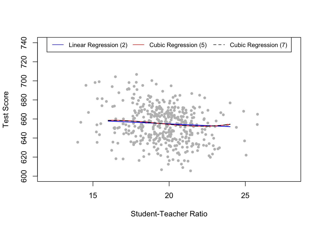
For the above figure all regressors except \(size\) are set to their sample averages. We see that the cubic regressions (5) and (7) are almost identical. They indicate that the relation between test scores and the student-teacher ratio only has a small amount of nonlinearity since they do not deviate much from the regression function of (2).
The next code chunk reproduces Figure 8.11 of the book. We use plot() and points() to color observations depending on \(HiEL\). Again, the regression lines are drawn based on predictions using average sample averages of all regressors except for \(size\).
# draw scatterplot

# observations with HiEL = 0
plot(CASchools$size[CASchools$HiEL == 0],
     CASchools$score[CASchools$HiEL == 0],
     xlim = c(12, 28),
     ylim = c(600, 730),
     pch = 20,
     col = "gray",
     xlab = "Student-Teacher Ratio",
     ylab = "Test Score")

# observations with HiEL = 1
points(CASchools$size[CASchools$HiEL == 1],
       CASchools$score[CASchools$HiEL == 1],
       col = "steelblue",
       pch = 20)

# add a legend
legend("top",
       legend = c("Regression (6) with HiEL=0", "Regression (6) with HiEL=1"),
       cex = 0.7,
       ncol = 2,
       lty = c(1, 1),
       col = c("green", "red"))

# data for use with 'predict()'
new_data <- data.frame("size" = seq(12, 28, 0.05),
                       "english" = mean(CASchools$english),
                       "lunch" = mean(CASchools$lunch),
                       "income" = mean(CASchools$income),
                       "HiEL" = 0)

# add estimated regression function for model (6) with HiEL=0
fitted <- predict(TestScore_mod6, newdata = new_data)

lines(new_data$size,
      fitted,
      lwd = 1.5,
      col = "green")

# add estimated regression function for model (6) with HiEL=1
new_data$HiEL <- 1

fitted <- predict(TestScore_mod6, newdata = new_data)

lines(new_data$size,
      fitted,
      lwd = 1.5,
      col = "red")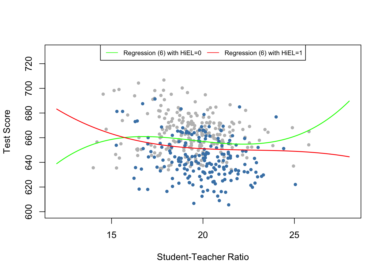
The regression output shows that model (6) finds statistically significant coefficients on the interaction terms \(HiEL:size\), \(HiEL:size^2\) and \(HiEL:size^3\), i.e., there is evidence that the nonlinear relationship connecting test scores and student-teacher ratio depends on the fraction of English learning students in the district. However, the above figure shows that this difference is not of practical importance and is a good example for why one should be careful when interpreting nonlinear models: although the two regression functions look different, we see that the slope of both functions is almost identical for student-teacher ratios between \(17\) and \(23\). Since this range includes almost \(90\%\) of all observations, we can be confident that nonlinear interactions between the fraction of English learners and the student-teacher ratio can be neglected.
One might be tempted to object since both functions show opposing slopes for student-teacher ratios below \(15\) and beyond \(24\). There are at least to possible objections:
There are only few observations with low and high values of the student-teacher ratio, so there is only little information to be exploited when estimating the model. This means the estimated function is less precise in the tails of the data set.
The above described behavior of the regression function, is a typical caveat when using cubic functions since they generally show extreme behavior for extreme regressor values. Think of the graph of \(f(x) = x^3\).
We thus find no clear evidence for a relation between class size and test scores on the percentage of English learners in the district.
Summary
We are now able to answer the three question posed at the beginning of this section.
In the linear models, the percentage of English learners has only little influence on the effect on test scores from changing the student-teacher ratio. This result stays valid if we control for economic background of the students. While the cubic specification (6) provides evidence that the effect the student-teacher ratio on test score depends on the share of English learners, the strength of this effect is negligible.
When controlling for the students’ economic background we find evidence of nonlinearities in the relationship between student-teacher ratio and test scores.
The linear specification (2) predicts that a reduction of the student-teacher ratio by two students per teacher leads to an improvement in test scores of about \(-0.73 \times (-2) = 1.46\) points. Since the model is linear, this effect is independent of the class size. Assume that the student-teacher ratio is \(20\). For example, the nonlinear model (5) predicts that the reduction increases test scores by \[64.33\cdot18+18^2\cdot(-3.42)+18^3\cdot(0.059) - (64.33\cdot20+20^2\cdot(-3.42)+20^3\cdot(0.059)) \approx 3.3\] points. If the ratio is \(22\), a reduction to \(20\) leads to a predicted improvement in test scores of \[64.33\cdot20+20^2\cdot(-3.42)+20^3\cdot(0.059) - (64.33\cdot22+22^2\cdot(-3.42)+22^3\cdot(0.059)) \approx 2.4\] points. This suggests that the effect is stronger in smaller classes.