15.1 The Orange Juice Data
The largest cultivation region for oranges in the U.S. is located in Florida which usually has ideal climate for the fruit growth. It thus is the source of almost all frozen juice concentrate produced in the country. However, from time to time and depending on their severeness, cold snaps cause a loss of harvests such that the supply of oranges decreases and consequently the price of frozen juice concentrate rises. The timing of the price increases is complicated: a cut in today’s supply of concentrate influences not just today’s price but also future prices because supply in future periods will decrease, too. Clearly, the magnitude of today’s and future prices increases due to freeze is an empirical question that can be investigated using a distributed lag model — a time series model that relates price changes to weather conditions.
To begin with the analysis, we reproduce Figure 15.1 of the book which displays plots of the price index for frozen concentrated orange juice, percentage changes in the price as well as monthly freezing degree days in Orlando, the center of Florida’s orange-growing region.
# load the frozen orange juice data set
data("FrozenJuice")

# compute the price index for frozen concentrated juice
FOJCPI <- FrozenJuice[, "price"]/FrozenJuice[, "ppi"]
FOJC_pctc <- 100 * diff(log(FOJCPI))
FDD <- FrozenJuice[, "fdd"]
# convert series to xts objects
FOJCPI_xts <- as.xts(FOJCPI)
FDD_xts <- as.xts(FrozenJuice[, 3])
# Plot orange juice price index
plot(as.zoo(FOJCPI),
col = "steelblue",
lwd = 2,
xlab = "Date",
ylab = "Price index",
main = "Frozen Concentrated Orange Juice")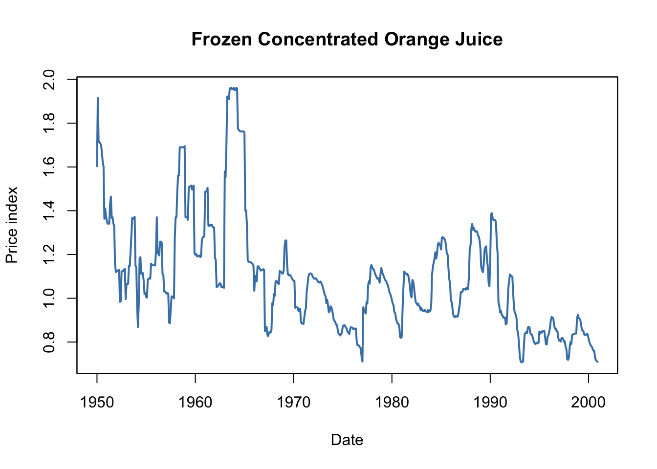
# divide plotting area
par(mfrow = c(2, 1))

# Plot percentage changes in prices
plot(as.zoo(FOJC_pctc),
     col = "steelblue",
     lwd = 2,
     xlab = "Date",
     ylab = "Percent",
     main = "Monthly Changes in the Price of Frozen Conentrated Orange Juice")

# plot freezing degree days
plot(as.zoo(FDD),
     col = "steelblue",
     lwd = 2,
     xlab = "Date",
     ylab = "Freezing degree days",
     main = "Monthly Freezing Degree Days in Orlando, FL")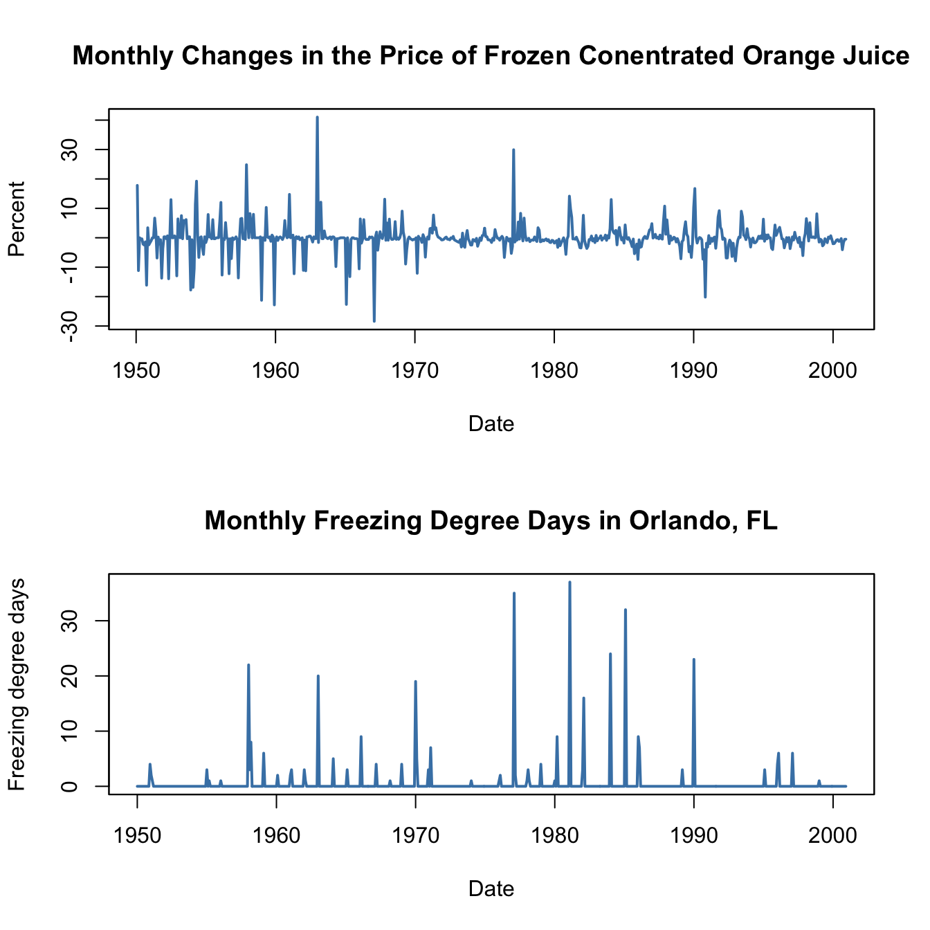
Periods with a high amount of freezing degree days are followed by large month-to-month price changes. These coinciding movements motivate a simple regression of price changes (\(\%ChgOJC_t\)) on freezing degree days (\(FDD_t\)) to estimate the effect of an additional freezing degree day one the price in the current month. For this, as for all other regressions in this chapter, we use \(T=611\) observations (January 1950 to December 2000).
# simple regression of percentage changes on freezing degree days
orange_SR <- dynlm(FOJC_pctc ~ FDD)
coeftest(orange_SR, vcov. = vcovHAC)
##
## t test of coefficients:
##
## Estimate Std. Error t value Pr(>|t|)
## (Intercept) -0.42095 0.18683 -2.2531 0.0246064 *
## FDD 0.46724 0.13385 3.4906 0.0005167 ***
## ---
## Signif. codes: 0 '***' 0.001 '**' 0.01 '*' 0.05 '.' 0.1 ' ' 1Notice that the standard errors are computed using a “HAC” estimator of the variance-covariance matrix, see Chapter 14.5 for a discussion of this estimator.
\[\begin{align*} \widehat{\%ChgOJC_t} = -\underset{(0.19)}{0.42} + \underset{(0.13)}{0.47} FDD_t \end{align*}\]The estimated coefficient on \(FDD_t\) has the following interpretation: an additional freezing degree day in month \(t\) leads to a price increase 0f \(0.47\) percentage points in the same month.
To consider effects of cold snaps on the orange juice price over the subsequent periods, we include lagged values of \(FDD_t\) in our model which leads to a distributed lag regression model. We estimate a specification using a contemporaneous and six lagged values of \(FDD_t\) as regressors.
# distributed lag model with 6 lags of freezing degree days
orange_DLM <- dynlm(FOJC_pctc ~ FDD + L(FDD, 1:6))
coeftest(orange_DLM, vcov. = vcovHAC)
##
## t test of coefficients:
##
## Estimate Std. Error t value Pr(>|t|)
## (Intercept) -0.692961 0.212445 -3.2618 0.0011700 **
## FDD 0.471433 0.135195 3.4871 0.0005242 ***
## L(FDD, 1:6)1 0.145021 0.081557 1.7782 0.0758853 .
## L(FDD, 1:6)2 0.058364 0.058911 0.9907 0.3222318
## L(FDD, 1:6)3 0.074166 0.047143 1.5732 0.1162007
## L(FDD, 1:6)4 0.036304 0.029335 1.2376 0.2163670
## L(FDD, 1:6)5 0.048756 0.031370 1.5543 0.1206535
## L(FDD, 1:6)6 0.050246 0.045129 1.1134 0.2659919
## ---
## Signif. codes: 0 '***' 0.001 '**' 0.01 '*' 0.05 '.' 0.1 ' ' 1As the result we obtain
\[\begin{align} \begin{split} \widehat{\%ChgOJC_t} =& -\underset{(0.21)}{0.69} + \underset{(0.14)}{0.47} FDD_t + \underset{(0.08)}{0.15} FDD_{t-1} + \underset{(0.06)}{0.06} FDD_{t-2} + \underset{(0.05)}{0.07} FDD_{t-3} \\ &+ \underset{(0.03)}{0.04} FDD_{t-4} + \underset{(0.03)}{0.05} FDD_{t-5} + \underset{(0.05)}{0.05} FDD_{t-6}, \end{split} \tag{15.1} \end{align}\]where the coefficient on \(FDD_{t-1}\) estimates the price increase in period \(t\) caused by an additional freezing degree day in the preceding month, the coefficient on \(FDD_{t-2}\) estimates the effect of an additional freezing degree day two month ago and so on. Consequently, the coefficients in (15.1) can be interpreted as price changes in current and future periods due to a unit increase in the current month’ freezing degree days.