7.5 Model Specification for Multiple Regression
Choosing a regression specification, i.e., selecting the variables to be included in a regression model, is a difficult task. However, there are some guidelines on how to proceed. The goal is clear: obtaining an unbiased and precise estimate of the causal effect of interest. As a starting point, think about omitted variables, that is, to avoid possible bias by using suitable control variables. Omitted variables bias in the context of multiple regression is explained in Key Concept 7.3. A second step could be to compare different specifications by measures of fit. However, as we shall see one should not rely solely on \(\bar{R}^2\).
Key Concept 7.3
Omitted Variable Bias in Multiple Regression
Omitted variable bias is the bias in the OLS estimator that arises when regressors correlate with an omitted variable. For omitted variable bias to arise, two things must be true:
- At least one of the included regressors must be correlated with the omitted variable.
- The omitted variable must be a determinant of the dependent variable, \(Y\).
We now discuss an example were we face a potential omitted variable bias in a multiple regression model:
Consider again the estimated regression equation
\[ \widehat{TestScore} = \underset{(8.7)}{686.0} - \underset{(0.43)}{1.10} \times size - \underset{(0.031)}{0.650} \times english. \]
We are interested in estimating the causal effect of class size on test score. There might be a bias due to omitting “outside learning opportunities” from our regression since such a measure could be a determinant of the students’ test scores and could also be correlated with both regressors already included in the model (so that both conditions of Key Concept 7.3 are fulfilled). “Outside learning opportunities” are a complicated concept that is difficult to quantify. A surrogate we can consider instead is the students’ economic background which likely are strongly related to outside learning opportunities: think of wealthy parents that are able to provide time and/or money for private tuition of their children. We thus augment the model with the variable lunch, the percentage of students that qualify for a free or subsidized lunch in school due to family incomes below a certain threshold, and reestimate the model.
# estimate the model and print the summary to console
model <- lm(score ~ size + english + lunch, data = CASchools)
coeftest(model, vcov. = vcovHC, type = "HC1")
##
## t test of coefficients:
##
## Estimate Std. Error t value Pr(>|t|)
## (Intercept) 700.149957 5.568453 125.7351 < 2.2e-16 ***
## size -0.998309 0.270080 -3.6963 0.0002480 ***
## english -0.121573 0.032832 -3.7029 0.0002418 ***
## lunch -0.547345 0.024107 -22.7046 < 2.2e-16 ***
## ---
## Signif. codes: 0 '***' 0.001 '**' 0.01 '*' 0.05 '.' 0.1 ' ' 1Thus, the estimated regression line is
\[ \widehat{TestScore} = \underset{(5.56)}{700.15} - \underset{(0.27)}{1.00} \times size - \underset{(0.03)}{0.12} \times english - \underset{(0.02)}{0.55} \times lunch. \]
We observe no substantial changes in the conclusion about the effect of \(size\) on \(TestScore\): the coefficient on \(size\) changes by only \(0.1\) and retains its significance.
Although the difference in estimated coefficients is not big in this case, it is useful to keep lunch to make the assumption of conditional mean independence more credible (see Chapter 7.5 of the book).
Model Specification in Theory and in Practice
Key Concept 7.4 lists some common pitfalls when using \(R^2\) and \(\bar{R}^2\) to evaluate the predictive ability of regression models.
Key Concept 7.4
\(R^2\) and \(\bar{R}^2\): what they tell you — and what they do not
The \(R^2\) and \(\bar{R}^2\) tell you whether the regressors are good at explaining the variation of the independent variable in the sample. If the \(R^2\) (or \(\bar{R}^2\)) is nearly \(1\), then the regressors produce a good prediction of the dependent variable in that sample, in the sense that the variance of OLS residuals is small compared to the variance of the dependent variable. If the \(R^2\) (or \(\bar{R}^2\)) is nearly \(0\), the opposite is true.
The \(R^2\) and \(\bar{R}^2\) do not tell you whether:
- An included variable is statistically significant.
- The regressors are the true cause of the movements in the dependent variable.
- There is omitted variable bias.
- You have chosen the most appropriate set of regressors.
For example, think of regressing \(TestScore\) on \(PLS\) which measures the available parking lot space in thousand square feet. You are likely to observe a significant coefficient of reasonable magnitude and moderate to high values for \(R^2\) and \(\bar{R}^2\). The reason for this is that parking lot space is correlated with many determinants of the test score like location, class size, financial endowment and so on. Although we do not have observations on \(PLS\), we can use R to generate some relatively realistic data.
# set seed for reproducibility
set.seed(1)

# generate observations for parking lot space
CASchools$PLS <- c(22 * CASchools$income
                   - 15 * CASchools$size
                   + 0.2 * CASchools$expenditure
                   + rnorm(nrow(CASchools), sd = 80) + 3000)
# plot parking lot space against test score
plot(CASchools$PLS,
CASchools$score,
xlab = "Parking Lot Space",
ylab = "Test Score",
pch = 20,
col = "steelblue")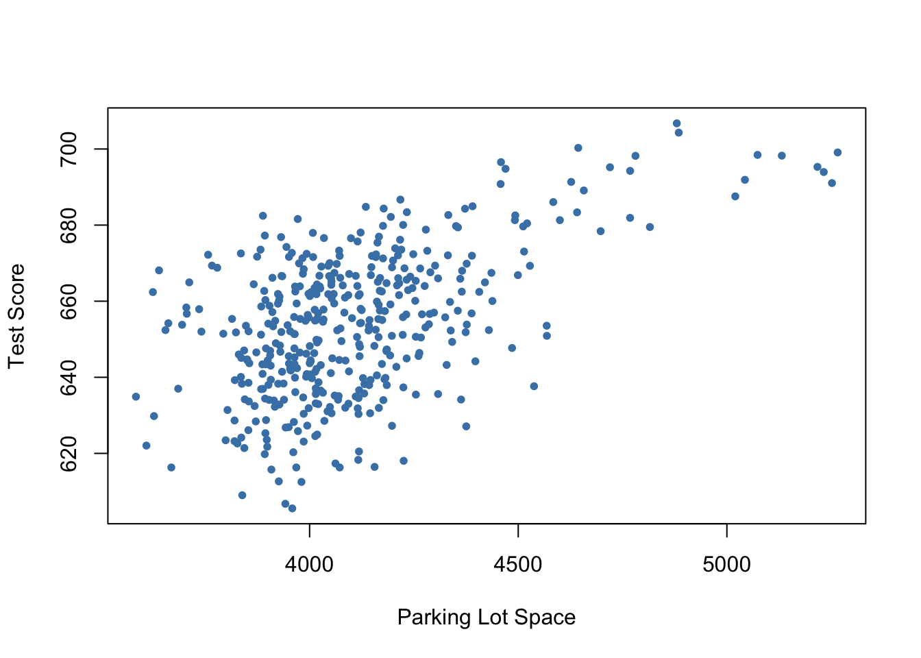
# regress test score on PLS
summary(lm(score ~ PLS, data = CASchools))
##
## Call:
## lm(formula = score ~ PLS, data = CASchools)
##
## Residuals:
## Min 1Q Median 3Q Max
## -42.608 -11.049 0.342 12.558 37.105
##
## Coefficients:
## Estimate Std. Error t value Pr(>|t|)
## (Intercept) 4.897e+02 1.227e+01 39.90 <2e-16 ***
## PLS 4.002e-02 2.981e-03 13.43 <2e-16 ***
## ---
## Signif. codes: 0 '***' 0.001 '**' 0.01 '*' 0.05 '.' 0.1 ' ' 1
##
## Residual standard error: 15.95 on 418 degrees of freedom
## Multiple R-squared: 0.3013, Adjusted R-squared: 0.2996
## F-statistic: 180.2 on 1 and 418 DF, p-value: < 2.2e-16using lm() we find that the coefficient on \(PLS\) is positive and significantly different from zero. Also \(R^2\) and \(\bar{R}^2\) are about \(0.3\) which is a lot more than the roughly \(0.05\) observed when regressing the test scores on the class sizes only. This suggests that increasing the parking lot space boosts a school’s test scores and that model (7.1) does even better in explaining heterogeneity in the dependent variable than a model with \(size\) as the only regressor. Keeping in mind how \(PLS\) is constructed this comes as no surprise. It is evident that the high \(R^2\)