2.1 Random Variables and Probability Distributions
Let us briefly review some basic concepts of probability theory.
- The mutually exclusive results of a random process are called the outcomes. ‘Mutually exclusive’ means that only one of the possible outcomes can be observed.
- We refer to the probability of an outcome as the proportion that the outcome occurs in the long run, that is, if the experiment is repeated very often.
- The set of all possible outcomes of a random variable is called the sample space.
- An event is a subset of the sample space and consists of one or more outcomes.
These ideas are unified in the concept of a random variable which is a numerical summary of random outcomes. Random variables can be discrete or continuous.
- Discrete random variables have discrete outcomes, e.g., \(0\) and \(1\).
- A continuous random variable may take on a continuum of possible values.
Probability Distributions of Discrete Random Variables
A typical example for a discrete random variable \(D\) is the result of a dice roll: in terms of a random experiment this is nothing but randomly selecting a sample of size \(1\) from a set of numbers which are mutually exclusive outcomes. Here, the sample space is \(\{1,2,3,4,5,6\}\) and we can think of many different events, e.g., ‘the observed outcome lies between \(2\) and \(5\)’.
A basic function to draw random samples from a specified set of elements is the the function sample(), see ?sample. We can use it to simulate the random outcome of a dice roll. Let’s roll the dice!
sample(1:6, 1) ## [1] 6The probability distribution of a discrete random variable is the list of all possible values of the variable and their probabilities which sum to \(1\). The cumulative probability distribution function gives the probability that the random variable is less than or equal to a particular value.
For the dice roll, the probability distribution and the cumulative probability distribution are summarized in Table 2.1.
| Outcome | 1 | 2 | 3 | 4 | 5 | 6 |
| Probability | 1/6 | 1/6 | 1/6 | 1/6 | 1/6 | 1/6 |
| Cumulative Probability | 1/6 | 2/6 | 3/6 | 4/6 | 5/6 | 1 |
We can easily plot both functions using R. Since the probability equals \(1/6\) for each outcome, we set up the vector probability by using the function rep() which replicates a given value a specified number of times.
# generate the vector of probabilities
probability <- rep(1/6, 6)

# plot the probabilites
plot(probability,
     main = "Probability Distribution",
xlab = "outcomes") 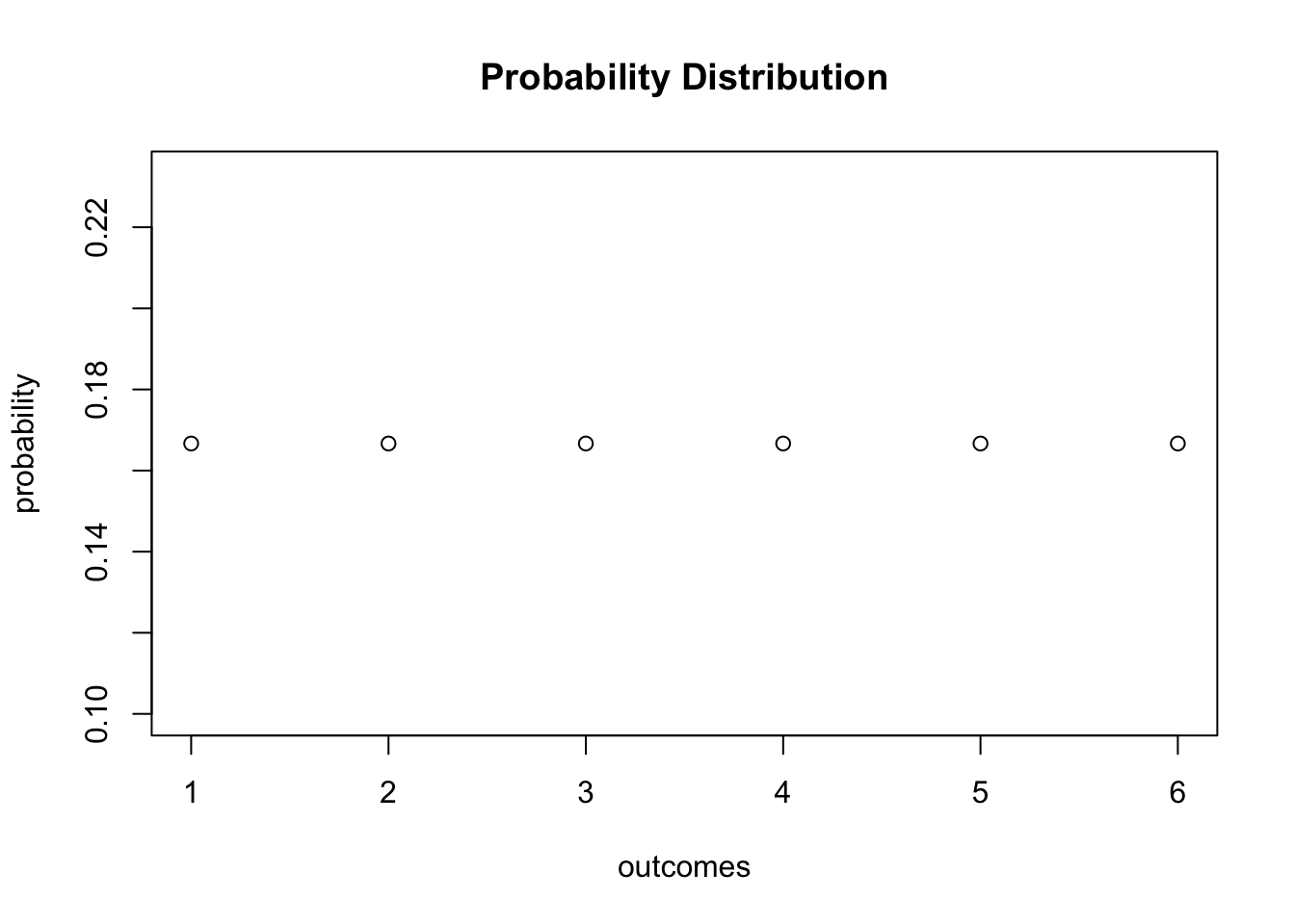
For the cumulative probability distribution we need the cumulative probabilities, i.e., we need the cumulative sums of the vector probability. These sums can be computed using cumsum().
# generate the vector of cumulative probabilities
cum_probability <- cumsum(probability)

# plot the probabilites
plot(cum_probability,
     xlab = "outcomes",
main = "Cumulative Probability Distribution") 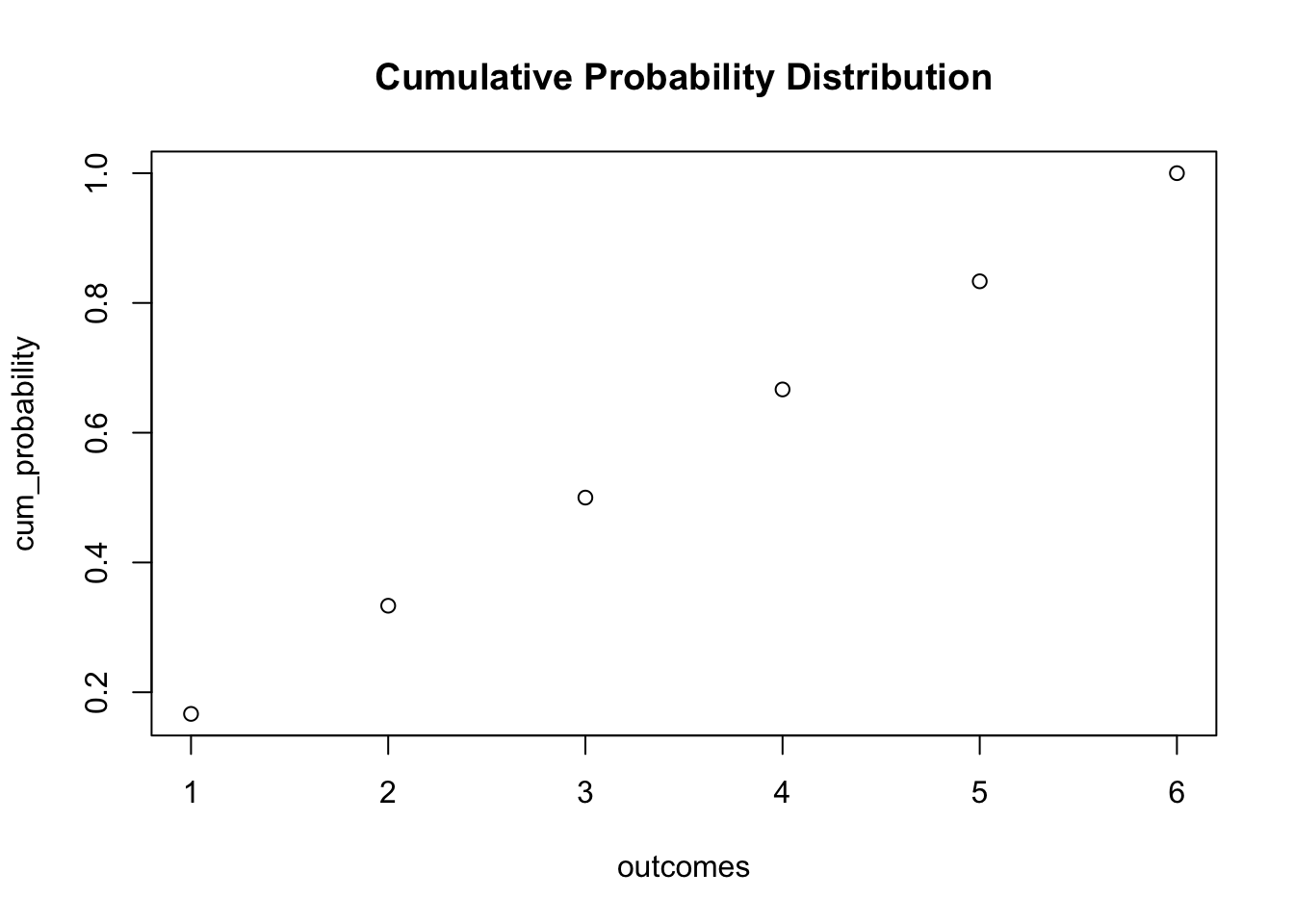
Bernoulli Trials
The set of elements from which sample() draws outcomes does not have to consist of numbers only. We might as well simulate coin tossing with outcomes \(H\) (heads) and \(T\) (tails).
sample(c("H", "T"), 1) ## [1] "H"The result of a single coin toss is a Bernoulli distributed random variable, i.e., a variable with two possible distinct outcomes.
Imagine you are about to toss a coin \(10\) times in a row and wonder how likely it is to end up with a \(5\) times heads. This is a typical example of what we call a Bernoulli experiment as it consists of \(n=10\) Bernoulli trials that are independent of each other and we are interested in the likelihood of observing \(k=5\) successes \(H\) that occur with probability \(p=0.5\) (assuming a fair coin) in each trial. Note that the order of the outcomes does not matter here.
It is a well known result that the number of successes \(k\) in a Bernoulli experiment follows a binomial distribution. We denote this as
\[k \sim B(n,p).\]
The probability of observing \(k\) successes in the experiment \(B(n,p)\) is given by
\[f(k)=P(k)=\begin{pmatrix}n\\ k \end{pmatrix} \cdot p^k \cdot (1-p)^{n-k}=\frac{n!}{k!(n-k)!} \cdot p^k \cdot (1-p)^{n-k}\]
with \(\begin{pmatrix}n\\ k \end{pmatrix}\) the binomial coefficient.
In R, we can solve the problem stated above by means of the function dbinom() which calculates the probability of the binomial distribution given the parameters x, size, and prob, see ?binom.
dbinom(x = 5,
       size = 10,
       prob = 0.5)
## [1] 0.2460938We conclude that the probability of observing Head \(k=5\) times when tossing the coin \(n=10\) times is about \(24.6\%\).
Now assume we are interested in \(P(4 \leq k \leq 7)\), i.e., the probability of observing \(4\), \(5\), \(6\) or \(7\) successes for \(B(10,0.5)\). This may be computed by providing a vector as the argument x in our call of dbinom() and summing up using sum().
# compute P(4 <= k <= 7) using 'dbinom()'
sum(dbinom(x = 4:7,
         size = 10,
         prob = 0.5))
## [1] 0.7734375An alternative approach is to use pbinom(), the distribution function of the binomial distribution to compute \[P(4 \leq k \leq 7) = P(k \leq 7) - P(k\leq3 ).\]
# compute P(4 <= k <= 7) using 'pbinom()'
pbinom(size = 10, prob = 0.5, q = 7) - pbinom(size = 10, prob = 0.5, q = 3)
## [1] 0.7734375The probability distribution of a discrete random variable is nothing but a list of all possible outcomes that can occur and their respective probabilities. In the coin tossing example we have \(11\) possible outcomes for \(k\).
# set up vector of possible outcomes
k <- 0:10
To visualize the probability distribution function of \(k\) we may therefore do the following:
# assign the probabilities
probability <- dbinom(x = k,
                      size = 10,
                      prob = 0.5)

# plot the outcomes against their probabilities
plot(x = k,
     y = probability,
main = "Probability Distribution Function") 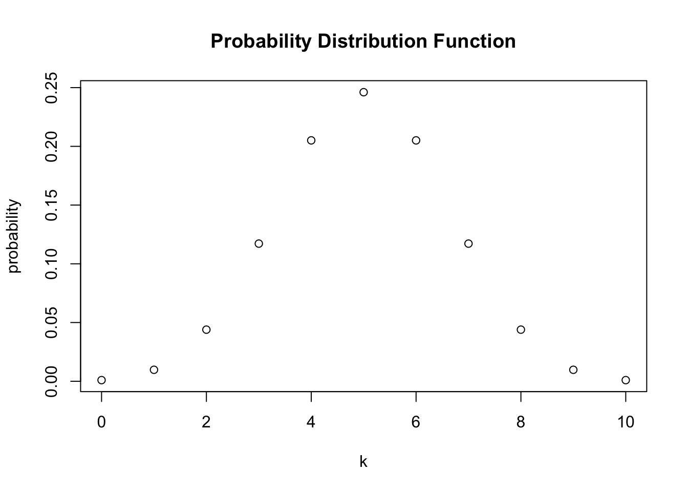
In a similar fashion we may plot the cumulative distribution function of \(k\) by executing the following code chunk:
# compute cumulative probabilities
prob <- dbinom(x = 0:10,
               size = 10,
               prob = 0.5)

# plot the cumulative probabilities
plot(x = k,
     y = prob,
main = "Cumulative Distribution Function") 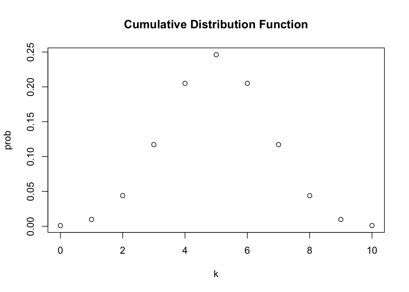
Expected Value, Mean and Variance
The expected value of a random variable is, loosely, the long-run average value of its outcomes when the number of repeated trials is large. For a discrete random variable, the expected value is computed as a weighted average of its possible outcomes whereby the weights are the related probabilities. This is formalized in Key Concept 2.1.
Key Concept 2.1
Expected Value and the Mean
Suppose the random variable \(Y\) takes on \(k\) possible values, \(y_1, \dots, y_k\), where \(y_1\) denotes the first value, \(y_2\) denotes the second value, and so forth, and that the probability that \(Y\) takes on \(y_1\) is \(p_1\), the probability that \(Y\) takes on \(y_2\) is \(p_2\) and so forth. The expected value of \(Y\), \(E(Y)\) is defined as
\[ E(Y) = y_1 p_1 + y_2 p_2 + \cdots + y_k p_k = \sum_{i=1}^k y_i p_i \]
where the notation \(\sum_{i=1}^k y_i p_i\) means “the sum of \(y_i\) \(p_i\) for \(i\) running from \(1\) to \(k\)”. The expected value of \(Y\) is also called the mean of \(Y\) or the expectation of \(Y\) and is denoted by \(\mu_Y\).In the dice example, the random variable, \(D\) say, takes on \(6\) possible values \(d_1 = 1, d_2 = 2, \dots, d_6 = 6\). Assuming a fair dice, each of the \(6\) outcomes occurs with a probability of \(1/6\). It is therefore easy to calculate the exact value of \(E(D)\) by hand:
\[ E(D) = 1/6 \sum_{i=1}^6 d_i = 3.5 \]
\(E(D)\) is simply the average of the natural numbers from \(1\) to \(6\) since all wights \(p_i\) are \(1/6\). This can be easily calculated using the function mean() which computes the arithmetic mean of a numeric vector.
# compute mean of natural numbers from 1 to 6
mean(1:6)
## [1] 3.5An example of sampling with replacement is rolling a dice three times in a row.
# set seed for reproducibility
set.seed(1)

# rolling a dice three times in a row
sample(1:6, 3, replace = T)
## [1] 2 3 4Of course we could also consider a much bigger number of trials, \(10000\) say. Doing so, it would be pointless to simply print the results to the console: by default R displays up to \(1000\) entries of large vectors and omits the remainder (give it a try). Eyeballing the numbers does not reveal much. Instead, let us calculate the sample average of the outcomes using mean() and see if the result comes close to the expected value \(E(D)=3.5\).
# set seed for reproducibility
set.seed(1)

# compute the sample mean of 10000 dice rolls
mean(sample(1:6,
           10000,
           replace = T))
## [1] 3.5039We find the sample mean to be fairly close to the expected value. This result will be discussed in Chapter 2.2 in more detail.
Other frequently encountered measures are the variance and the standard deviation. Both are measures of the dispersion of a random variable.
Key Concept 2.2
Variance and Standard Deviation
The variance of the discrete random variable \(Y\), denoted \(\sigma^2_Y\), is \[ \sigma^2_Y = \text{Var}(Y) = E\left[(Y-\mu_y)^2\right] = \sum_{i=1}^k (y_i - \mu_y)^2 p_i \] The standard deviation of \(Y\) is \(\sigma_Y\), the square root of the variance. The units of the standard deviation are the same as the units of \(Y\).
The variance as defined in Key Concept 2.2, being a population quantity, is not implemented as a function in R. Instead we have the function var() which computes the sample variance
\[ s^2_Y = \frac{1}{n-1} \sum_{i=1}^n (y_i - \overline{y})^2. \]
Remember that \(s^2_Y\) is different from the so called population variance of a discrete random variable \(Y\),
\[ \text{Var}(Y) = \frac{1}{N} \sum_{i=1}^N (y_i - \mu_Y)^2. \]
since it measures how the data is dispersed around the sample average \(\overline{y}\) instead of the population mean \(\mu_Y\). This becomes clear when we look at our dice rolling example. For \(D\) we have
\[ \text{Var}(D) = 1/6 \sum_{i=1}^6 (d_i - 3.5)^2 = 2.92 \] which is obviously different from the result of \(s^2\) as computed by var().
var(1:6)## [1] 3.5The sample variance as computed by var() is an estimator of the population variance. You may check this using the widget below.
Probability Distributions of Continuous Random Variables
Since a continuous random variable takes on a continuum of possible values, we cannot use the concept of a probability distribution as used for discrete random variables. Instead, the probability distribution of a continuous random variable is summarized by its probability density function (PDF).
The cumulative probability distribution function (CDF) for a continuous random variable is defined just as in the discrete case. Hence, the cumulative probability distribution of a continuous random variables states the probability that the random variable is less than or equal to a particular value.
For completeness, we present revisions of Key Concepts 2.1 and 2.2 for the continuous case.
Key Concept 2.3
Probabilities, Expected Value and Variance of a Continuous Random Variable
Let \(f_Y(y)\) denote the probability density function of \(Y\). The probability that \(Y\) falls between \(a\) and \(b\) where \(a < b\) is \[ P(a \leq Y \leq b) = \int_a^b f_Y(y) \mathrm{d}y. \] We further have that \(P(-\infty \leq Y \leq \infty) = 1\) and therefore \(\int_{-\infty}^{\infty} f_Y(y) \mathrm{d}y = 1\).
As for the discrete case, the expected value of \(Y\) is the probability weighted average of its values. Due to continuity, we use integrals instead of sums. The expected value of \(Y\) is defined as
\[ E(Y) = \mu_Y = \int y f_Y(y) \mathrm{d}y. \]
The variance is the expected value of \((Y - \mu_Y)^2\). We thus have
\[\text{Var}(Y) = \sigma_Y^2 = \int (y - \mu_Y)^2 f_Y(y) \mathrm{d}y.\]Let us discuss an example:
Consider the continuous random variable \(X\) with probability density function
\[ f_X(x) = \frac{3}{x^4}, x>1. \]
- We can show analytically that the integral of \(f_X(x)\) over the real line equals \(1\).
- The expectation of \(X\) can be computed as follows:
- Note that the variance of \(X\) can be expressed as \(\text{Var}(X) = E(X^2) - E(X)^2\). Since \(E(X)\) has been computed in the previous step, we seek \(E(X^2)\):
So we have shown that the area under the curve equals one, that the expectation is \(E(X)=\frac{3}{2} \ \) and we found the variance to be \(\text{Var}(X) = \frac{3}{4}\). However, this was tedious and, as we shall see, an analytic approach is not applicable for some probability density functions, e.g., if integrals have no closed form solutions.
Luckily, R also enables us to easily find the results derived above. The tool we use for this is the function integrate(). First, we have to define the functions we want to calculate integrals for as R functions, i.e., the PDF \(f_X(x)\) as well as the expressions \(x\cdot f_X(x)\) and \(x^2\cdot f_X(x)\).
# define functions
f <- function(x) 3 / x^4
g <- function(x) x * f(x)
h <- function(x) x^2 * f(x)
Next, we use integrate() and set lower and upper limits of integration to \(1\) and \(\infty\) using arguments lower and upper. By default, integrate() prints the result along with an estimate of the approximation error to the console. However, the outcome is not a numeric value one can readily do further calculation with. In order to get only a numeric value of the integral, we need to use the \(</tt> operator in conjunction with <tt>value</tt>. The <tt>\) operator is used to extract elements by name from an object of type list.
# compute area under the density curve
area <- integrate(f,
                 lower = 1,
                 upper = Inf)$value
area
## [1] 1# compute E(X)
EX <- integrate(g,
lower = 1,
upper = Inf)$value
EX## [1] 1.5# compute Var(X)
VarX <- integrate(h,
lower = 1,
upper = Inf)$value - EX^2
VarX## [1] 0.75Although there is a wide variety of distributions, the ones most often encountered in econometrics are the normal, chi-squared, Student \(t\) and \(F\) distributions. Therefore we will discuss some core R functions that allow to do calculations involving densities, probabilities and quantiles of these distributions.
Every probability distribution that R handles has four basic functions whose names consist of a prefix followed by a root name. As an example, take the normal distribution. The root name of all four functions associated with the normal distribution is norm. The four prefixes are
- d for “density” - probability function / probability density function
- p for “probability” - cumulative distribution function
- q for “quantile” - quantile function (inverse cumulative distribution function)
- r for “random” - random number generator
Thus, for the normal distribution we have the R functions dnorm(), pnorm(), qnorm() and rnorm().
The Normal Distribution
The probably most important probability distribution considered here is the normal distribution. This is not least due to the special role of the standard normal distribution and the Central Limit Theorem which is to be treated shortly. Normal distributions are symmetric and bell-shaped. A normal distribution is characterized by its mean \(\mu\) and its standard deviation \(\sigma\), concisely expressed by \(\mathcal{N}(\mu,\sigma^2)\). The normal distribution has the PDF
\[\begin{align} f(x) = \frac{1}{\sqrt{2 \pi} \sigma} \exp{-(x - \mu)^2/(2 \sigma^2)}. \end{align}\]For the standard normal distribution we have \(\mu=0\) and \(\sigma=1\). Standard normal variates are often denoted by \(Z\). Usually, the standard normal PDF is denoted by \(\phi\) and the standard normal CDF is denoted by \(\Phi\). Hence, \[ \phi(c) = \Phi'(c) \ \ , \ \ \Phi(c) = P(Z \leq c) \ \ , \ \ Z \sim \mathcal{N}(0,1).\] In R, we can conveniently obtain densities of normal distributions using the function dnorm(). Let us draw a plot of the standard normal density function using curve() in conjunction with dnorm().
# draw a plot of the N(0,1) PDF
curve(dnorm(x),
      xlim = c(-3.5, 3.5),
      ylab = "Density",
main = "Standard Normal Density Function") 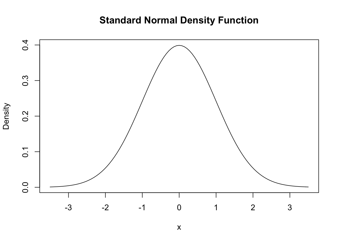
We can obtain the density at different positions by passing a vector to dnorm().
# compute denstiy at x=-1.96, x=0 and x=1.96
dnorm(x = c(-1.96, 0, 1.96))
## [1] 0.05844094 0.39894228 0.05844094Similar to the PDF, we can plot the standard normal CDF using curve(). We could use dnorm() for this but it is much more convenient to rely on pnorm().
# plot the standard normal CDF
curve(pnorm(x),
      xlim = c(-3.5, 3.5),
      ylab = "Density",
      main = "Standard Normal Cumulative Distribution Function")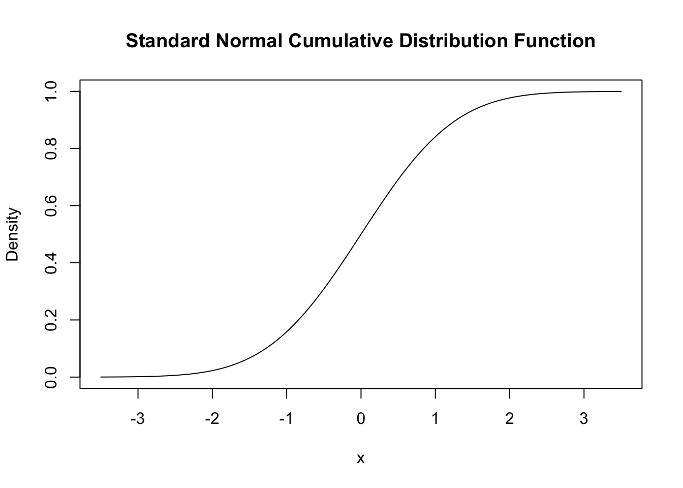
We can also use R to calculate the probability of events associated with a standard normal variate.
Let us say we are interested in \(P(Z \leq 1.337)\). For some continuous random variable \(Z\) on \([-\infty,\infty]\) with density \(g(x)\) we would have to determine \(G(x)\), the anti-derivative of \(g(x)\) so that
\[ P(Z \leq 1.337 ) = G(1.337) = \int_{-\infty}^{1.337} g(x) \mathrm{d}x. \]
If \(Z \sim \mathcal{N}(0,1)\), we have \(g(x)=\phi(x)\). There is no analytic solution to the integral above. Fortunately, R offers good approximations. The first approach makes use of the function integrate() which allows to solve one-dimensional integration problems using a numerical method. For this, we first define the function we want to compute the integral of as an R function f. In our example, f is the standard normal density function and hence takes a single argument x. Following the definition of \(\phi(x)\) we define f as
# define the standard normal PDF as an R function
f <- function(x) {
  1/(sqrt(2 * pi)) * exp(-0.5 * x^2)
}
Let us check if this function computes standard normal densities by passing a vector.
# define a vector of reals
quants <- c(-1.96, 0, 1.96)

# compute densities
f(quants)
## [1] 0.05844094 0.39894228 0.05844094# compare to the results produced by 'dnorm()'
f(quants) == dnorm(quants)## [1] TRUE TRUE TRUEThe results produced by f() are indeed equivalent to those given by dnorm().
Next, we call integrate() on f() and specify the arguments lower and upper, the lower and upper limits of integration.
# integrate f()
integrate(f,
          lower = -Inf,
          upper = 1.337)
## 0.9093887 with absolute error < 1.7e-07We find that the probability of observing \(Z \leq 1.337\) is about \(0.9094\%\).
A second and much more convenient way is to use the function pnorm(), the standard normal cumulative distribution function.
# compute the probability using pnorm()
pnorm(1.337)
## [1] 0.9093887The result matches the outcome of the approach using integrate().
Let us discuss some further examples:
A commonly known result is that \(95\%\) probability mass of a standard normal lies in the interval \([-1.96, 1.96]\), that is, in a distance of about \(2\) standard deviations to the mean. We can easily confirm this by calculating \[ P(-1.96 \leq Z \leq 1.96) = 1-2\times P(Z \leq -1.96) \] due to symmetry of the standard normal PDF. Thanks to R, we can abandon the table of the standard normal CDF found in many other textbooks and instead solve this fast by using pnorm().
# compute the probability
1 - 2 * (pnorm(-1.96))
## [1] 0.9500042To make statements about the probability of observing outcomes of \(Y\) in some specific range is more convenient when we standardize first as shown in Key Concept 2.4.
Key Concept 2.4
Computing Probabilities Involving Normal Random Variables
Suppose \(Y\) is normally distributed with mean \(\mu\) and variance \(\sigma^2\): \[Y \sim \mathcal{N}(\mu, \sigma^2)\] Then \(Y\) is standardized by subtracting its mean and dividing by its standard deviation: \[ Z = \frac{Y -\mu}{\sigma} \] Let \(c_1\) and \(c_2\) denote two numbers whereby \(c_1 < c_2\) and further \(d_1 = (c_1 - \mu) / \sigma\) and \(d_2 = (c_2 - \mu)/\sigma\). Then
\[\begin{align*} P(Y \leq c_2) =& \, P(Z \leq d_2) = \Phi(d_2), \\ P(Y \geq c_1) =& \, P(Z \geq d_1) = 1 - \Phi(d_1), \\ P(c_1 \leq Y \leq c_2) =& \, P(d_1 \leq Z \leq d_2) = \Phi(d_2) - \Phi(d_1). \end{align*}\]Now consider a random variable \(Y\) with \(Y \sim \mathcal{N}(5, 25)\). R functions that handle the normal distribution can perform the standardization. If we are interested in \(P(3 \leq Y \leq 4)\) we can use pnorm() and adjust for a mean and/or a standard deviation that deviate from \(\mu=0\) and \(\sigma = 1\) by specifying the arguments mean and sd accordingly. Attention: the argument sd requires the standard deviation, not the variance!
pnorm(4, mean = 5, sd = 5) - pnorm(3, mean = 5, sd = 5) ## [1] 0.07616203An extension of the normal distribution in a univariate setting is the multivariate normal distribution. The joint PDF of two random normal variables \(X\) and \(Y\) is given by
\[\begin{align} \begin{split} g_{X,Y}(x,y) =& \, \frac{1}{2\pi\sigma_X\sigma_Y\sqrt{1-\rho_{XY}^2}} \\ \cdot & \, \exp \left\{ \frac{1}{-2(1-\rho_{XY}^2)} \left[ \left( \frac{x-\mu_x}{\sigma_X} \right)^2 - 2\rho_{XY}\left( \frac{x-\mu_X}{\sigma_X} \right)\left( \frac{y-\mu_Y}{\sigma_Y} \right) + \left( \frac{y-\mu_Y}{\sigma_Y} \right)^2 \right] \right\}. \end{split} \tag{2.1} \end{align}\]Equation (2.1) contains the bivariate normal PDF. It is somewhat hard to gain insights from this complicated expression. Instead, let us consider the special case where \(X\) and \(Y\) are uncorrelated standard normal random variables with densities \(f_X(x)\) and \(f_Y(y)\) with joint normal distribution. We then have the parameters \(\sigma_X = \sigma_Y = 1\), \(\mu_X=\mu_Y=0\) (due to marginal standard normality) and \(\rho_{XY}=0\) (due to independence). The joint density of \(X\) and \(Y\) then becomes
\[ g_{X,Y}(x,y) = f_X(x) f_Y(y) = \frac{1}{2\pi} \cdot \exp \left\{ -\frac{1}{2} \left[x^2 + y^2 \right] \right\}, \tag{2.2} \]
the PDF of the bivariate standard normal distribution. The widget below provides an interactive three-dimensional plot of (2.2).
By moving the cursor over the plot you can see that the density is rotationally invariant, i.e., the density at \((a, b)\) solely depends on the distance of \((a, b)\) to the origin: geometrically, regions of equal density are edges of concentric circles in the \(XY\)-plane, centered at \((\mu_X = 0, \mu_Y = 0)\).
The normal distribution has some remarkable characteristics. For example, for two jointly normally distribued variables \(X\) and \(Y\), the conditional expectation function is linear: one can show that \[ E(Y\vert X) = E(Y) + \rho \frac{\sigma_Y}{\sigma_X} (X - E(X)). \] The application below shows standard bivariate normally distributed sample data along with the conditional expectation function \(E(Y\vert X)\) and the marginal densities of \(X\) and \(Y\). All elements adjust accordingly as you vary the parameters.
The Chi-Squared Distribution
The chi-squared distribution is another distribution relevant in econometrics. It is often needed when testing special types of hypotheses frequently encountered when dealing with regression models.
The sum of \(M\) squared independent standard normal distributed random variables follows a chi-squared distribution with \(M\) degrees of freedom:
\[\begin{align*} Z_1^2 + \dots + Z_M^2 = \sum_{m=1}^M Z_m^2 \sim \chi^2_M \ \ \text{with} \ \ Z_m \overset{i.i.d.}{\sim} \mathcal{N}(0,1) \tag{2.2} \end{align*}\]A \(\chi^2\) distributed random variable with \(M\) degrees of freedom has expectation \(M\), mode at \(M-2\) for \(M \geq 2\) and variance \(2 \cdot M\). For example, for
\[ Z_1,Z_2,Z_3 \overset{i.i.d.}{\sim} \mathcal{N}(0,1) \]
it holds that
\[ Z_1^2+Z_2^2+Z_3^3 \sim \chi^2_3. \tag{2.3} \] Using the code below, we can display the PDF and the CDF of a \(\chi^2_3\) random variable in a single plot. This is achieved by setting the argument add = TRUE in the second call of curve(). Further we adjust limits of both axes using xlim and ylim and choose different colors to make both functions better distinguishable. The plot is completed by adding a legend with help of legend().
# plot the PDF
curve(dchisq(x, df = 3),
      xlim = c(0, 10),
      ylim = c(0, 1),
      col = "blue",
      ylab = "",
      main = "p.d.f. and c.d.f of Chi-Squared Distribution, M = 3")

# add the CDF to the plot
curve(pchisq(x, df = 3),
      xlim = c(0, 10),
      add = TRUE,
      col = "red")

# add a legend to the plot
legend("topleft",
       c("PDF", "CDF"),
       col = c("blue", "red"),
       lty = c(1, 1))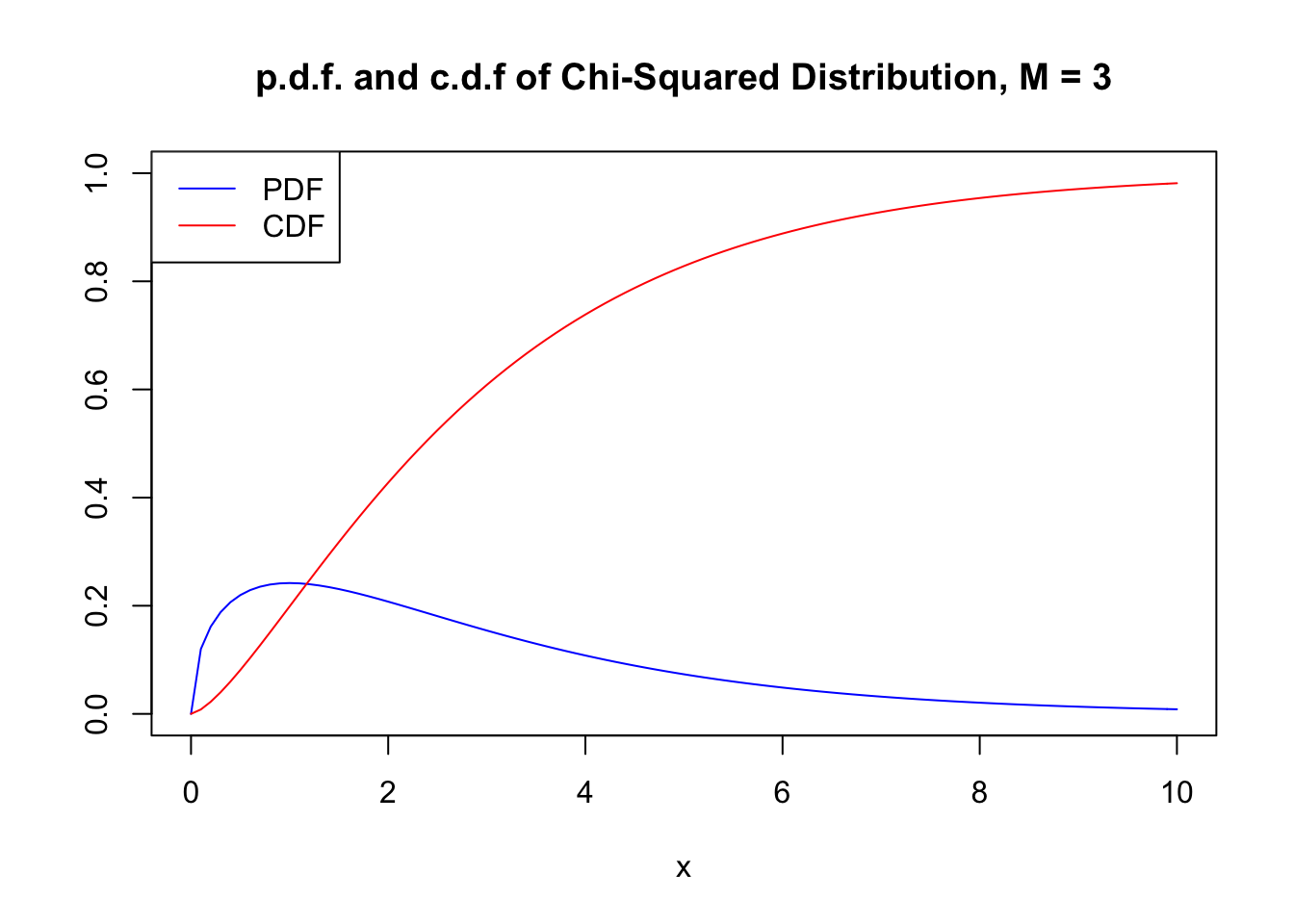
Since the outcomes of a \(\chi^2_M\) distributed random variable are always positive, the support of the related PDF and CDF is \(\mathbb{R}_{\geq0}\).
As expectation and variance depend (solely!) on the degrees of freedom, the distribution’s shape changes drastically if we vary the number of squared standard normals that are summed up. This relation is often depicted by overlaying densities for different \(M\), see the Wikipedia Article.
We reproduce this here by plotting the density of the \(\chi_1^2\) distribution on the interval \([0,15]\) with curve(). In the next step, we loop over degrees of freedom \(M=2,...,7\) and add a density curve for each \(M\) to the plot. We also adjust the line color for each iteration of the loop by setting col = M. At last, we add a legend that displays degrees of freedom and the associated colors.
# plot the density for M=1
curve(dchisq(x, df = 1),
      xlim = c(0, 15),
      xlab = "x",
      ylab = "Density",
      main = "Chi-Square Distributed Random Variables")

# add densities for M=2,...,7 to the plot using a 'for()' loop
for (M in 2:7) {
  curve(dchisq(x, df = M),
        xlim = c(0, 15),
        add = T,
        col = M)
}

# add a legend
legend("topright",
       as.character(1:7),
       col = 1:7 ,
       lty = 1,
       title = "D.F.")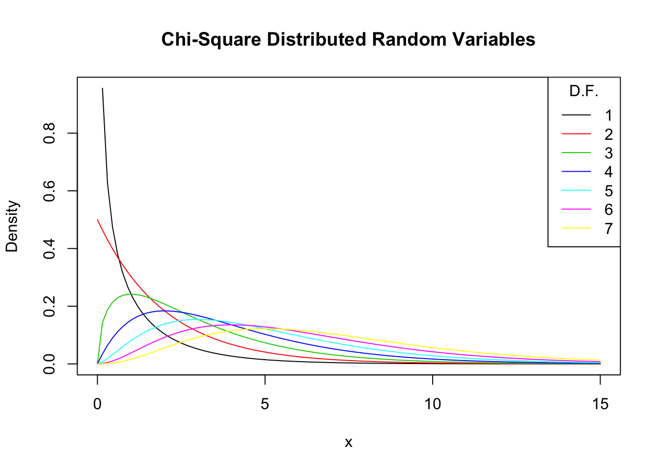
Increasing the degrees of freedom shifts the distribution to the right (the mode becomes larger) and increases the dispersion (the distribution’s variance grows).
The Student t Distribution
Let \(Z\) be a standard normal variate, \(W\) a \(\chi^2_M\) random variable and further assume that \(Z\) and \(W\) are independent. Then it holds that
\[ \frac{Z}{\sqrt{W/M}} =:X \sim t_M \] and \(X\) follows a Student \(t\) distribution (or simply \(t\) distribution) with \(M\) degrees of freedom.
Similar to the \(\chi^2_M\) distribution, the shape of a \(t_M\) distribution depends on \(M\). \(t\) distributions are symmetric, bell-shaped and look similar to a normal distribution, especially when \(M\) is large. This is not a coincidence: for a sufficiently large \(M\), the \(t_M\) distribution can be approximated by the standard normal distribution. This approximation works reasonably well for \(M\geq 30\). As we will illustrate later by means of a small simulation study, the \(t_{\infty}\) distribution is the standard normal distribution.
A \(t_M\) distributed random variable \(X\) has an expectation if \(M>1\) and it has a variance if \(M>2\).
\[\begin{align} E(X) =& 0, \ M>1 \\ \text{Var}(X) =& \frac{M}{M-2}, \ M>2 \end{align}\]Let us plot some \(t\) distributions with different \(M\) and compare them to the standard normal distribution.
# plot the standard normal density
curve(dnorm(x),
      xlim = c(-4, 4),
      xlab = "x",
      lty = 2,
      ylab = "Density",
      main = "Densities of t Distributions")

# plot the t density for M=2
curve(dt(x, df = 2),
      xlim = c(-4, 4),
      col = 2,
      add = T)

# plot the t density for M=4
curve(dt(x, df = 4),
      xlim = c(-4, 4),
      col = 3,
      add = T)

# plot the t density for M=25
curve(dt(x, df = 25),
      xlim = c(-4, 4),
      col = 4,
      add = T)

# add a legend
legend("topright",
       c("N(0, 1)", "M=2", "M=4", "M=25"),
       col = 1:4,
       lty = c(2, 1, 1, 1))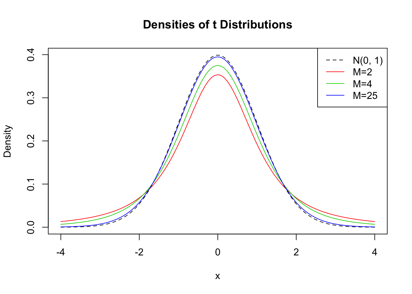
The plot illustrates what has been said in the previous paragraph: as the degrees of freedom increase, the shape of the \(t\) distribution comes closer to that of a standard normal bell curve. Already for \(M=25\) we find little difference to the standard normal density. If \(M\) is small, we find the distribution to have heavier tails than a standard normal, i.e., it has a “fatter” bell shape.
The F Distribution
Another ratio of random variables important to econometricians is the ratio of two independent \(\chi^2\) distributed random variables that are divided by their degrees of freedom \(M\) and \(n\). The quantity
\[ \frac{W/M}{V/n} \sim F_{M,n} \ \ \text{with} \ \ W \sim \chi^2_M \ \ , \ \ V \sim \chi^2_n \] follows an \(F\) distribution with numerator degrees of freedom \(M\) and denominator degrees of freedom \(n\), denoted \(F_{M,n}\). The distribution was first derived by George Snedecor but was named in honor of Sir Ronald Fisher.
By definition, the support of both PDF and CDF of an \(F_{M,n}\) distributed random variable is \(\mathbb{R}_{\geq0}\).
Say we have an \(F\) distributed random variable \(Y\) with numerator degrees of freedom \(3\) and denominator degrees of freedom \(14\) and are interested in \(P(Y \geq 2)\). This can be computed with help of the function pf(). By setting the argument lower.tail to TRUE we ensure that R computes \(1- P(Y \leq 2)\), i.e,the probability mass in the tail right of \(2\).
pf(2, 3, 13, lower.tail = F)## [1] 0.1638271We can visualize this probability by drawing a line plot of the related density and adding a color shading with polygon().
# define coordinate vectors for vertices of the polygon
x <- c(2, seq(2, 10, 0.01), 10)
y <- c(0, df(seq(2, 10, 0.01), 3, 14), 0)

# draw density of F_{3, 14}
curve(df(x ,3 ,14),
      ylim = c(0, 0.8),
      xlim = c(0, 10),
      ylab = "Density",
      main = "Density Function")

# draw the polygon
polygon(x, y, col = "orange")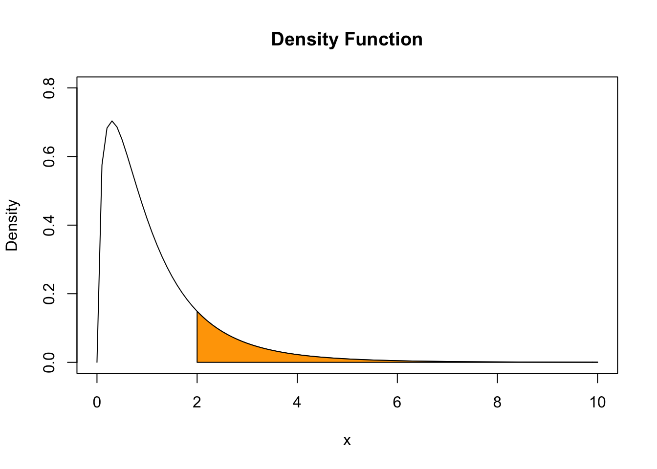
The \(F\) distribution is related to many other distributions. An important special case encountered in econometrics arises if the denominator degrees of freedom are large such that the \(F_{M,n}\) distribution can be approximated by the \(F_{M,\infty}\) distribution which turns out to be simply the distribution of a \(\chi^2_M\) random variable divided by its degrees of freedom \(M\),
\[ W/M \sim F_{M,\infty} \ \ , \ \ W \sim \chi^2_M. \]