16.1 Vector Autoregressions
A Vector autoregressive (VAR) model is useful when one is interested in predicting multiple time series variables using a single model. At its core, the VAR model is an extension of the univariate autoregressive model we have dealt with in Chapters 14 and 15. Key Concept 16.1 summarizes the essentials of VAR.
Key Concept
16.1
Vector Autoregressions
The vector autoregression (VAR) model extends the idea of univariate autoregression to \(k\) time series regressions, where the lagged values of all \(k\) series appear as regressors. Put differently, in a VAR model we regress a vector of time series variables on lagged vectors of these variables. As for AR(\(p\)) models, the lag order is denoted by \(p\) so the VAR(\(p\)) model of two variables \(X_t\) and \(Y_t\) (\(k=2\)) is given by the equations
\[\begin{align*} Y_t =& \, \beta_{10} + \beta_{11} Y_{t-1} + \dots + \beta_{1p} Y_{t-p} + \gamma_{11} X_{t-1} + \dots + \gamma_{1p} X_{t-p} + u_{1t}, \\ X_t =& \, \beta_{20} + \beta_{21} Y_{t-1} + \dots + \beta_{2p} Y_{t-p} + \gamma_{21} X_{t-1} + \dots + \gamma_{2p} X_{t-p} + u_{2t}. \end{align*}\]The \(\beta\)s and \(\gamma\)s can be estimated using OLS on each equation. The assumptions for VARs are the time series assumptions presented in Key Concept 14.6 applied to each of the equations.
It is straightforward to estimate VAR models in R. A feasible approach is to simply use lm() for estimation of the individual equations. Furthermore, the Rpackage vars provides standard tools for estimation, diagnostic testing and prediction using this type of models.
When the assumptions of Key Concept 16.1 hold, the OLS estimators of the VAR coefficients are consistent and jointly normal in large samples so that the usual inferential methods such as confidence intervals and \(t\)-statistics can be used.
The structure of VARs also allows to jointly test restrictions across multiple equations. For instance, it may be of interest to test whether the coefficients on all regressors of the lag \(p\) are zero. This corresponds to testing the null that the lag order \(p-1\) is correct. Large sample joint normality of the coefficient estimates is convenient because it implies that we may simply use an \(F\)-test for this testing problem. The explicit formula for such a test statistic is rather complicated but fortunately such computations are easily done using the R functions we work with in this chapter. Another way to determine optimal lag lengths are information criteria like the \(BIC\) which we have introduced for univariate time series regressions in Chapter 14.6. Just as in the case of a single equation, for a multiple equation model we choose the specification which has the smallest \(BIC(p)\), where \[\begin{align*} BIC(p) =& \, \log\left[\text{det}(\widehat{\Sigma}_u)\right] + k(kp+1) \frac{\log(T)}{T}. \end{align*}\]with \(\widehat{\Sigma}_u\) denoting the estimate of the \(k \times k\) covariance matrix of the VAR errors and \(\text{det}(\cdot)\) denotes the determinant.
As for univariate distributed lag models, one should think carefully about variables to include in a VAR, as adding unrelated variables reduces the forecast accuracy by increasing the estimation error. This is particularly important because the number of parameters to be estimated grows qudratically to the number of variables modeled by the VAR. In the application below we shall see that economic theory and empirical evidence are helpful for this decision.
A VAR Model of the Growth Rate of GDP and the Term Spread
We now show how to estimate a VAR model of the GDP growth rate, \(GDPGR\), and the term spread, \(TSpread\). As following the discussion on nonstationarity of GDP growth in Chapter 14.7 (recall the possible break in the early 1980s detected by the \(QLR\) test statistic), we use data from 1981:Q1 to 2012:Q4. The two model equations are
\[\begin{align*} GDPGR_t =& \, \beta_{10} + \beta_{11} GDPGR_{t-1} + \beta_{12} GDPGR_{t-2} + \gamma_{11} TSpread_{t-1} + \gamma_{12} TSpread_{t-2} + u_{1t}, \\ TSpread_t =& \, \beta_{20} + \beta_{21} GDPGR_{t-1} + \beta_{22} GDPGR_{t-2} + \gamma_{21} TSpread_{t-1} + \gamma_{22} TSpread_{t-2} + u_{2t}. \end{align*}\]The data set us_macro_quarterly.xlsx is provided on the companion website to J. Stock & Watson (2015) and can be downloaded here. It contains quarterly data on U.S. real (i.e., inflation adjusted) GDP from 1947 to 2004. We begin by importing the data set and do some formatting (we already worked with this data set in Chapter 14 so you may skip these steps if you have already loaded the data in your working environment).
# load the U.S. macroeconomic data set
USMacroSWQ <- read_xlsx("Data/us_macro_quarterly.xlsx",
                         sheet = 1,
                         col_types = c("text", rep("numeric", 9)))

# set the column names
colnames(USMacroSWQ) <- c("Date", "GDPC96", "JAPAN_IP", "PCECTPI", "GS10",
                          "GS1", "TB3MS", "UNRATE", "EXUSUK", "CPIAUCSL")

# format the date column
USMacroSWQ$Date <- as.yearqtr(USMacroSWQ$Date, format = "%Y:0%q")

# define GDP as ts object
GDP <- ts(USMacroSWQ$GDPC96,
          start = c(1957, 1),
          end = c(2013, 4),
          frequency = 4)

# define GDP growth as a ts object
GDPGrowth <- ts(400*log(GDP[-1]/GDP[-length(GDP)]),
                start = c(1957, 2),
                end = c(2013, 4),
                frequency = 4)

# 3-months Treasury bill interest rate as a 'ts' object
TB3MS <- ts(USMacroSWQ$TB3MS,
            start = c(1957, 1),
            end = c(2013, 4),
            frequency = 4)

# 10-years Treasury bonds interest rate as a 'ts' object
TB10YS <- ts(USMacroSWQ$GS10,
              start = c(1957, 1),
              end = c(2013, 4),
              frequency = 4)

# generate the term spread series
TSpread <- TB10YS - TB3MS
We estimate both equations separately by OLS and use coeftest() to obtain robust standard errors.
# Estimate both equations using 'dynlm()'
VAR_EQ1 <- dynlm(GDPGrowth ~ L(GDPGrowth, 1:2) + L(TSpread, 1:2),
                 start = c(1981, 1),
                 end = c(2012, 4))

VAR_EQ2 <- dynlm(TSpread ~ L(GDPGrowth, 1:2) + L(TSpread, 1:2),
                 start = c(1981, 1),
                 end = c(2012, 4))

# rename regressors for better readability
names(VAR_EQ1$coefficients) <- c("Intercept","Growth_t-1",
                                 "Growth_t-2", "TSpread_t-1", "TSpread_t-2")
names(VAR_EQ2$coefficients) <- names(VAR_EQ1$coefficients)

# robust coefficient summaries
coeftest(VAR_EQ1, vcov. = sandwich)
##
## t test of coefficients:
##
## Estimate Std. Error t value Pr(>|t|)
## Intercept 0.516344 0.524429 0.9846 0.3267616
## Growth_t-1 0.289553 0.110827 2.6127 0.0101038 *
## Growth_t-2 0.216392 0.085879 2.5197 0.0130255 *
## TSpread_t-1 -0.902549 0.358290 -2.5190 0.0130498 *
## TSpread_t-2 1.329831 0.392660 3.3867 0.0009503 ***
## ---
## Signif. codes: 0 '***' 0.001 '**' 0.01 '*' 0.05 '.' 0.1 ' ' 1coeftest(VAR_EQ2, vcov. = sandwich)##
## t test of coefficients:
##
## Estimate Std. Error t value Pr(>|t|)
## Intercept 0.4557740 0.1214227 3.7536 0.0002674 ***
## Growth_t-1 0.0099785 0.0218424 0.4568 0.6485920
## Growth_t-2 -0.0572451 0.0264099 -2.1676 0.0321186 *
## TSpread_t-1 1.0582279 0.0983750 10.7571 < 2.2e-16 ***
## TSpread_t-2 -0.2191902 0.1086198 -2.0180 0.0457712 *
## ---
## Signif. codes: 0 '***' 0.001 '**' 0.01 '*' 0.05 '.' 0.1 ' ' 1We end up with the following results:
\[\begin{align*} GDPGR_t =& \, \underset{(0.46)}{0.52} + \underset{(0.11)}{0.29} GDPGR_{t-1} + \underset{(0.09)}{0.22} GDPGR_{t-2} -\underset{(0.36)}{0.90} TSpread_{t-1} + \underset{(0.39)}{1.33} TSpread_{t-2} \\ TSpread_t =& \, \underset{(0.12)}{0.46} + \underset{(0.02)}{0.01} GDPGR_{t-1} -\underset{(0.03)}{0.06} GDPGR_{t-2} + \underset{(0.10)}{1.06} TSpread_{t-1} -\underset{(0.11)}{0.22} TSpread_{t-2} \end{align*}\]The function VAR() can be used to obtain the same coefficient estimates as presented above since it applies OLS per equation, too.
# set up data for estimation using `VAR()`
VAR_data <- window(ts.union(GDPGrowth, TSpread), start = c(1980, 3), end = c(2012, 4))

# estimate model coefficients using `VAR()`
VAR_est <- VAR(y = VAR_data, p = 2)
VAR_est
##
## VAR Estimation Results:
## =======================
##
## Estimated coefficients for equation GDPGrowth:
## ==============================================
## Call:
## GDPGrowth = GDPGrowth.l1 + TSpread.l1 + GDPGrowth.l2 + TSpread.l2 + const
##
## GDPGrowth.l1 TSpread.l1 GDPGrowth.l2 TSpread.l2 const
## 0.2895533 -0.9025493 0.2163919 1.3298305 0.5163440
##
##
## Estimated coefficients for equation TSpread:
## ============================================
## Call:
## TSpread = GDPGrowth.l1 + TSpread.l1 + GDPGrowth.l2 + TSpread.l2 + const
##
## GDPGrowth.l1 TSpread.l1 GDPGrowth.l2 TSpread.l2 const
## 0.009978489 1.058227945 -0.057245123 -0.219190243 0.455773969VAR() returns a list of lm objects which can be passed to the usual functions, for example summary() and so it is straightforward to obtain model statistics for the individual equations.
# obtain the adj. R^2 from the output of 'VAR()'
summary(VAR_est$varresult$GDPGrowth)$adj.r.squared
## [1] 0.2887223summary(VAR_est$varresult$TSpread)$adj.r.squared## [1] 0.8254311We may use the individual model objects to conduct Granger causality tests.
# Granger causality tests:

# test if term spread has no power in explaining GDP growth
linearHypothesis(VAR_EQ1,
                 hypothesis.matrix = c("TSpread_t-1", "TSpread_t-2"),
                 vcov. = sandwich)
## Linear hypothesis test
##
## Hypothesis:
## TSpread_t - 0
## TSpread_t - 2 = 0
##
## Model 1: restricted model
## Model 2: GDPGrowth ~ L(GDPGrowth, 1:2) + L(TSpread, 1:2)
##
## Note: Coefficient covariance matrix supplied.
##
## Res.Df Df F Pr(>F)
## 1 125
## 2 123 2 5.9094 0.003544 **
## ---
## Signif. codes: 0 '***' 0.001 '**' 0.01 '*' 0.05 '.' 0.1 ' ' 1# test if GDP growth has no power in explaining term spread
linearHypothesis(VAR_EQ2,
hypothesis.matrix = c("Growth_t-1", "Growth_t-2"),
vcov. = sandwich)## Linear hypothesis test
##
## Hypothesis:
## Growth_t - 0
## Growth_t - 2 = 0
##
## Model 1: restricted model
## Model 2: TSpread ~ L(GDPGrowth, 1:2) + L(TSpread, 1:2)
##
## Note: Coefficient covariance matrix supplied.
##
## Res.Df Df F Pr(>F)
## 1 125
## 2 123 2 3.4777 0.03395 *
## ---
## Signif. codes: 0 '***' 0.001 '**' 0.01 '*' 0.05 '.' 0.1 ' ' 1Both Granger causality tests reject at the level of \(5\%\). This is evidence in favor of the conjecture that the term spread has power in explaining GDP growth and vice versa.
Iterated Multivariate Forecasts using an Iterated VAR
The idea of an iterated forecast for period \(T+2\) based on observations up to period \(T\) is to use the one-period-ahead forecast as an intermediate step. That is, the forecast for period \(T+1\) is used as an observation when predicting the level of a series for period \(T+2\). This can be generalized to a \(h\)-period-ahead forecast where all intervening periods between \(T\) and \(T+h\) must be forecasted as they are used as observations in the process (see Chapter 16.2 of the book for a more detailed argument on this concept). Iterated multiperiod forecasts are summarized in Key Concept 16.2.
Key Concept
16.2
Iterated Multiperiod Forecasts
The steps for an iterated multiperiod AR forecast are:
Estimate the AR(\(p\)) model using OLS and compute the one-period-ahead forecast.
Use the one-period-ahead forecast to obtain the two-period-ahead forecast.
Continue by iterating to obtain forecasts farther into the future.
An iterated multiperiod VAR forecast is done as follows:
Estimate the VAR(\(p\)) model using OLS per equation and compute the one-period-ahead forecast for all variables in the VAR.
Use the one-period-ahead forecasts to obtain the two-period-ahead forecasts.
Continue by iterating to obtain forecasts of all variables in the VAR farther into the future.
Since a VAR models all variables using lags of the respective other variables, we need to compute forecasts for all variables. It can be cumbersome to do so when the VAR is large but fortunately there are R functions that facilitate this. For example, the function predict() can be used to obtain iterated multivariate forecasts for VAR models estimated by the function VAR().
The following code chunk shows how to compute iterated forecasts for GDP growth and the term spread up to period 2015:Q1, that is \(h=10\), using the model object VAR_est.
# compute iterated forecasts for GDP growth and term spread for the next 10 quarters
forecasts <- predict(VAR_est)
forecasts
## $GDPGrowth
## fcst lower upper CI
## [1,] 1.738653 -3.006124 6.483430 4.744777
## [2,] 1.692193 -3.312731 6.697118 5.004925
## [3,] 1.911852 -3.282880 7.106583 5.194731
## [4,] 2.137070 -3.164247 7.438386 5.301317
## [5,] 2.329667 -3.041435 7.700769 5.371102
## [6,] 2.496815 -2.931819 7.925449 5.428634
## [7,] 2.631849 -2.846390 8.110088 5.478239
## [8,] 2.734819 -2.785426 8.255064 5.520245
## [9,] 2.808291 -2.745597 8.362180 5.553889
## [10,] 2.856169 -2.722905 8.435243 5.579074
##
## $TSpread
## fcst lower upper CI
## [1,] 1.676746 0.708471226 2.645021 0.9682751
## [2,] 1.884098 0.471880228 3.296316 1.4122179
## [3,] 1.999409 0.336348101 3.662470 1.6630609
## [4,] 2.080836 0.242407507 3.919265 1.8384285
## [5,] 2.131402 0.175797245 4.087008 1.9556052
## [6,] 2.156094 0.125220562 4.186968 2.0308738
## [7,] 2.161783 0.085037834 4.238528 2.0767452
## [8,] 2.154170 0.051061544 4.257278 2.1031082
## [9,] 2.138164 0.020749780 4.255578 2.1174139
## [10,] 2.117733 -0.007139213 4.242605 2.1248722This reveals that the two-quarter-ahead forecast of GDP growth in 2013:Q2 using data through 2012:Q4 is \(1.69\). For the same period, the iterated VAR forecast for the term spread is \(1.88\).
The matrices returned by predict(VAR_est) also include \(95\%\) prediction intervals (however, the function does not adjust for autocorrelation or heteroskedasticity of the errors!).
We may also plot the iterated forecasts for both variables by calling plot() on the output of predict(VAR_est).
# visualize the iterated forecasts
plot(forecasts)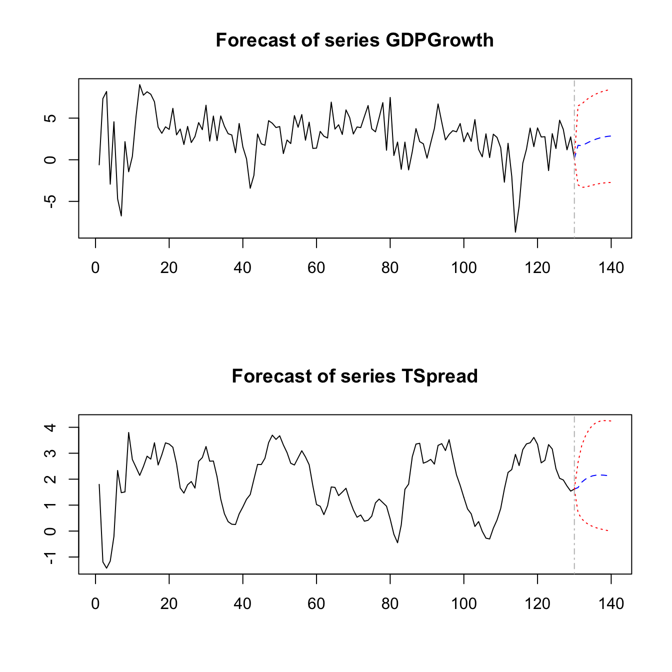
Direct Multiperiod Forecasts
A direct multiperiod forecast uses a model where the predictors are lagged appropriately such that the available observations can be used directly to do the forecast. The idea of direct multiperiod forecasting is summarized in Key Concept 16.3.
Key Concept
16.3
Direct Multiperiod Forecasts
A direct multiperiod forecast that forecasts \(h\) periods into the future using a model of \(Y_t\) and an additional predictor \(X_t\) with \(p\) lags is done by first estimating
\[\begin{align*} Y_t =& \, \delta_0 + \delta_1 Y_{t-h} + \dots + \delta_{p} Y_{t-p-h+1} + \delta_{p+1} X_{t-h} \\ +& \dots + \delta_{2p} Y_{t-p-h+1} + u_t, \end{align*}\] which is then used to compute the forecast of \(Y_{T+h}\) based on observations through period \(T\).For example, to obtain two-quarter-ahead forecasts of GDP growth and the term spread we first estimate the equations
\[\begin{align*} GDPGR_t =& \, \beta_{10} + \beta_{11} GDPGR_{t-2} + \beta_{12} GDPGR_{t-3} + \gamma_{11} TSpread_{t-2} + \gamma_{12} TSpread_{t-3} + u_{1t}, \\ TSpread_t =& \, \beta_{20} + \beta_{21} GDPGR_{t-2} + \beta_{22} GDPGR_{t-3} + \gamma_{21} TSpread_{t-2} + \gamma_{22} TSpread_{t-3} + u_{2t} \end{align*}\]and then substitute the values of \(GDPGR_{2012:Q4}\), \(GDPGR_{2012:Q3}\), \(TSpread_{2012:Q4}\) and \(TSpread_{2012:Q3}\) into both equations. This is easily done manually.
# estimate models for direct two-quarter-ahead forecasts
VAR_EQ1_direct <- dynlm(GDPGrowth ~ L(GDPGrowth, 2:3) + L(TSpread, 2:3),
                        start = c(1981, 1), end = c(2012, 4))

VAR_EQ2_direct <- dynlm(TSpread ~ L(GDPGrowth, 2:3) + L(TSpread, 2:3),
                        start = c(1981, 1), end = c(2012, 4))

# compute direct two-quarter-ahead forecasts
coef(VAR_EQ1_direct) %*% c(1, # intercept
                           window(GDPGrowth, start = c(2012, 3), end = c(2012, 4)),
                           window(TSpread, start = c(2012, 3), end = c(2012, 4)))
## [,1]
## [1,] 2.439497coef(VAR_EQ2_direct) %*% c(1, # intercept
window(GDPGrowth, start = c(2012, 3), end = c(2012, 4)),
window(TSpread, start = c(2012, 3), end = c(2012, 4)))## [,1]
## [1,] 1.66578Applied economists often use the iterated method since this forecasts are more reliable in terms of \(MSFE\), provided that the one-period-ahead model is correctly specified. If this is not the case, for example because one equation in a VAR is believed to be misspecified, it can be beneficial to use direct forecasts since the iterated method will then be biased and thus have a higher \(MSFE\) than the direct method. See Chapter 16.2 for a more detailed discussion on advantages and disadvantages of both methods.
References
Stock, J., & Watson, M. (2015). Introduction to Econometrics, Third Update, Global Edition. Pearson Education Limited.