15.6 Orange Juice Prices and Cold Weather
This section investigates the following two questions using the time series regression methods discussed here:
How persistent is the effect of a single freeze on orange juice concentrate prices?
Has the effect been stable over the whole time span?
We start by estimating dynamic causal effects with a distributed lag model where \(\%ChgOJC_t\) is regressed on \(FDD_t\) and 18 lags. A second model specification considers a transformation of the the distributed lag model which allows to estimate the 19 cumulative dynamic multipliers using OLS. The third model, adds 11 binary variables (one for each of the months from February to December) to adjust for a possible omitted variable bias arising from correlation of \(FDD_t\) and seasons by adding season(FDD) to the right hand side of the formula of the second model.
# estimate distributed lag models of frozen orange juice price changes
FOJC_mod_DM <- dynlm(FOJC_pctc ~ L(FDD, 0:18))
FOJC_mod_CM1 <- dynlm(FOJC_pctc ~ L(d(FDD), 0:17) + L(FDD, 18))
FOJC_mod_CM2 <- dynlm(FOJC_pctc ~ L(d(FDD), 0:17) + L(FDD, 18) + season(FDD))
The above models include a large number of lags with default labels that correspond to the degree of differencing and the lag orders which makes it somewhat cumbersome to read the output. The regressor labels of a model object may be altered by overriding the attribute names of the coefficient section using the function attr(). Thus, for better readability we use the lag orders as regressor labels.
# set lag orders as regressor labels
attr(FOJC_mod_DM$coefficients, "names")[1:20] <- c("(Intercept)", as.character(0:18))
attr(FOJC_mod_CM1$coefficients, "names")[1:20] <- c("(Intercept)", as.character(0:18))
attr(FOJC_mod_CM2$coefficients, "names")[1:20] <- c("(Intercept)", as.character(0:18))
Next, we compute HAC standard errors standard errors for each model using NeweyWest() and gather the results in a list which is then supplied as the argument se to the function stargazer(), see below. The sample consists of 612 observations:
length(FDD)## [1] 612According to (15.6), the rule of thumb for choosing the HAC standard error truncation parameter \(m\), we choose \[m = \left\lceil0.75 \cdot 612^{1/3} \right\rceil = \lceil6.37\rceil = 7.\] To check for sensitivity of the standard errors to different choices of the truncation parameter in the model that is used to estimate the cumulative multipliers, we also compute the Newey-West estimator for \(m=14\).
# gather HAC standard error errors in a list
SEs <- list(sqrt(diag(NeweyWest(FOJC_mod_DM, lag = 7, prewhite = F))),
            sqrt(diag(NeweyWest(FOJC_mod_CM1, lag = 7, prewhite = F))),
            sqrt(diag(NeweyWest(FOJC_mod_CM1, lag = 14, prewhite = F))),
            sqrt(diag(NeweyWest(FOJC_mod_CM2, lag = 7, prewhite = F))))
The results are then used to reproduce the outcomes presented in Table 15.1 of the book.
stargazer(FOJC_mod_DM , FOJC_mod_CM1, FOJC_mod_CM1, FOJC_mod_CM2,
  title = "Dynamic Effects of a Freezing Degree Day on the Price of Orange Juice",
  header = FALSE,
  digits = 3,
  column.labels = c("Dynamic Multipliers", rep("Dynamic Cumulative Multipliers", 3)),
  dep.var.caption  = "Dependent Variable: Monthly Percentage Change in Orange Juice Price",
  dep.var.labels.include = FALSE,
  covariate.labels = as.character(0:18),
  omit = "season",
  se = SEs,
  no.space = T,
  add.lines = list(c("Monthly indicators?","no", "no", "no", "yes"),
                   c("HAC truncation","7", "7", "14", "7")),
omit.stat = c("rsq", "f","ser")) | Dependent Variable: Monthly Percentage Change in Orange Juice Price | ||||
| Dynamic Multipliers | Dynamic Cumulative Multipliers | Dynamic Cumulative Multipliers | Dynamic Cumulative Multipliers | |
| (1) | (2) | (3) | (4) | |
| 0 | 0.508*** | 0.508*** | 0.508*** | 0.524*** |
| (0.137) | (0.137) | (0.139) | (0.142) | |
| 1 | 0.172** | 0.680*** | 0.680*** | 0.720*** |
| (0.088) | (0.134) | (0.130) | (0.142) | |
| 2 | 0.068 | 0.748*** | 0.748*** | 0.781*** |
| (0.060) | (0.165) | (0.162) | (0.173) | |
| 3 | 0.070 | 0.819*** | 0.819*** | 0.861*** |
| (0.044) | (0.181) | (0.181) | (0.190) | |
| 4 | 0.022 | 0.841*** | 0.841*** | 0.892*** |
| (0.031) | (0.183) | (0.184) | (0.194) | |
| 5 | 0.027 | 0.868*** | 0.868*** | 0.904*** |
| (0.030) | (0.189) | (0.189) | (0.199) | |
| 6 | 0.031 | 0.900*** | 0.900*** | 0.922*** |
| (0.047) | (0.202) | (0.208) | (0.210) | |
| 7 | 0.015 | 0.915*** | 0.915*** | 0.939*** |
| (0.015) | (0.205) | (0.210) | (0.212) | |
| 8 | -0.042 | 0.873*** | 0.873*** | 0.904*** |
| (0.034) | (0.214) | (0.218) | (0.219) | |
| 9 | -0.010 | 0.862*** | 0.862*** | 0.884*** |
| (0.051) | (0.236) | (0.245) | (0.239) | |
| 10 | -0.116* | 0.746*** | 0.746*** | 0.752*** |
| (0.069) | (0.257) | (0.262) | (0.259) | |
| 11 | -0.067 | 0.680** | 0.680** | 0.677** |
| (0.052) | (0.266) | (0.272) | (0.267) | |
| 12 | -0.143* | 0.537** | 0.537** | 0.551** |
| (0.076) | (0.268) | (0.271) | (0.272) | |
| 13 | -0.083* | 0.454* | 0.454* | 0.491* |
| (0.043) | (0.267) | (0.273) | (0.275) | |
| 14 | -0.057 | 0.397 | 0.397 | 0.427 |
| (0.035) | (0.273) | (0.284) | (0.278) | |
| 15 | -0.032 | 0.366 | 0.366 | 0.406 |
| (0.028) | (0.276) | (0.287) | (0.280) | |
| 16 | -0.005 | 0.360 | 0.360 | 0.408 |
| (0.055) | (0.283) | (0.293) | (0.286) | |
| 17 | 0.003 | 0.363 | 0.363 | 0.395 |
| (0.018) | (0.287) | (0.294) | (0.290) | |
| 18 | 0.003 | 0.366 | 0.366 | 0.386 |
| (0.017) | (0.293) | (0.301) | (0.295) | |
| Constant | -0.343 | -0.343 | -0.343 | -0.241 |
| (0.269) | (0.269) | (0.256) | (0.934) | |
| Monthly indicators? | no | no | no | yes |
| HAC truncation | 7 | 7 | 14 | 7 |
| Observations | 594 | 594 | 594 | 594 |
| Adjusted R2 | 0.109 | 0.109 | 0.109 | 0.101 |
| Note: | *p<0.1; **p<0.05; ***p<0.01 | |||
Table 15.1: Dynamic Effects of a Freezing Degree Day on the Price of Orange Juice
According to column (1) of Table 15.1, the contemporaneous effect of a freezing degree day is an increase of \(0.5\%\) in orange juice prices. The estimated effect is only \(0.17\%\) for the next month and close to zero for subsequent months. In fact, for all lags larger than 1, we cannot reject the null hypotheses that the respective coefficients are zero using individual \(t\)-tests. The model FOJC_mod_DM only explains little of the variation in the dependent variable (\(\bar{R}^2 = 0.11\)).
Columns (2) and (3) present estimates of the dynamic cumulative multipliers of model FOJC_mod_CM1. Apparently, it does not matter whether we choose \(m=7\) or \(m=14\) when computing HAC standard errors so we stick with \(m=7\) and the standard errors reported in column (2).
If the demand for orange juice is higher in winter, \(FDD_t\) would be correlated with the error term since freezes occur rather in winter so we would face omitted variable bias. The third model estimate, FOJC_mod_CM2, accounts for this possible issue by using an additional set of 11 monthly dummies. For brevity, estimates of the dummy coefficients are excluded from the output produced by stargazer (this is achieved by setting omit = ‘season’). We may check that the dummy for January was omitted to prevent perfect multicollinearity.
# estimates on mothly dummies
FOJC_mod_CM2$coefficients[-c(1:20)]
## season(FDD)Feb season(FDD)Mar season(FDD)Apr season(FDD)May season(FDD)Jun
## -0.9565759 -0.6358007 0.5006770 -1.0801764 0.3195624
## season(FDD)Jul season(FDD)Aug season(FDD)Sep season(FDD)Oct season(FDD)Nov
## 0.1951113 0.3644312 -0.4130969 -0.1566622 0.3116534
## season(FDD)Dec
## 0.1481589A comparison of the estimates presented in columns (3) and (4) indicates that adding monthly dummies has a negligible effect. Further evidence for this comes from a joint test of the hypothesis that the 11 dummy coefficients are zero. Instead of using linearHypothesis(), we use the function waldtest() and supply two model objects instead: unres_model, the unrestricted model object which is the same as FOJC_mod_CM2 (except for the coefficient names since we have modified them above) and res_model, the model where the restriction that all dummy coefficients are zero is imposed. res_model is conveniently obtained using the function update(). It extracts the argument formula of a model object, updates it as specified and then re-fits the model. By setting formula = . ~ . - season(FDD) we impose that the monthly dummies do not enter the model.
# test if coefficients on monthly dummies are zero
unres_model <- dynlm(FOJC_pctc ~ L(d(FDD), 0:17) + L(FDD, 18) + season(FDD))

res_model <- update(unres_model, formula = . ~ . - season(FDD))

waldtest(unres_model,
         res_model,
         vcov = NeweyWest(unres_model, lag = 7, prewhite = F))
## Wald test
##
## Model 1: FOJC_pctc ~ L(d(FDD), 0:17) + L(FDD, 18) + season(FDD)
## Model 2: FOJC_pctc ~ L(d(FDD), 0:17) + L(FDD, 18)
## Res.Df Df F Pr(>F)
## 1 563
## 2 574 -11 0.9683 0.4743The \(p\)-value is \(0.47\) so we cannot reject the hypothesis that the coefficients on the monthly dummies are zero, even at the \(10\%\) level. We conclude that the seasonal fluctuations in demand for orange juice do not pose a serious threat to internal validity of the model.
It is convenient to use plots of dynamic multipliers and cumulative dynamic multipliers. The following two code chunks reproduce Figures 15.2 (a) and 15.2 (b) of the book which display point estimates of dynamic and cumulative multipliers along with upper and lower bounds of their \(95\%\) confidence intervals computed using the above HAC standard errors.
# 95% CI bounds
point_estimates <- FOJC_mod_DM$coefficients

CI_bounds <- cbind("lower" = point_estimates - 1.96 * SEs[[1]],
                   "upper" = point_estimates + 1.96 * SEs[[1]])[-1, ]

# plot the estimated dynamic multipliers
plot(0:18, point_estimates[-1],
     type = "l",
     lwd = 2,
     col = "steelblue",
     ylim = c(-0.4, 1),
     xlab = "Lag",
     ylab = "Dynamic multiplier",
     main = "Dynamic Effect of FDD on Orange Juice Price")

# add a dashed line at 0
abline(h = 0, lty = 2)

# add CI bounds
lines(0:18, CI_bounds[,1], col = "darkred")
lines(0:18, CI_bounds[,2], col = "darkred")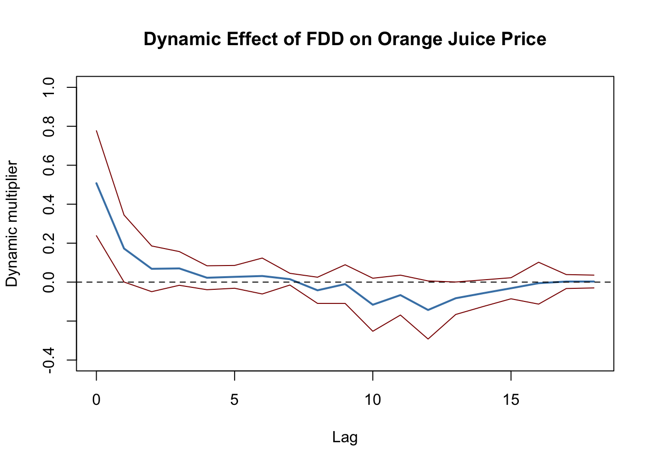
Figure 15.1: Dynamic Multipliers
The \(95\%\) confidence intervals plotted in Figure 15.1 indeed include zero for lags larger than 1 such that the null of a zero multiplier cannot be rejected for these lags.
# 95% CI bounds
point_estimates <- FOJC_mod_CM1$coefficients

CI_bounds <- cbind("lower" = point_estimates - 1.96 * SEs[[2]],
                   "upper" = point_estimates + 1.96 * SEs[[2]])[-1,]


# plot estimated dynamic multipliers
plot(0:18, point_estimates[-1],
     type = "l",
     lwd = 2,
     col = "steelblue",
     ylim = c(-0.4, 1.6),
     xlab = "Lag",
     ylab = "Cumulative dynamic multiplier",
     main = "Cumulative Dynamic Effect of FDD on Orange Juice Price")

# add dashed line at 0
abline(h = 0, lty = 2)

# add CI bounds
lines(0:18, CI_bounds[, 1], col = "darkred")
lines(0:18, CI_bounds[, 2], col = "darkred")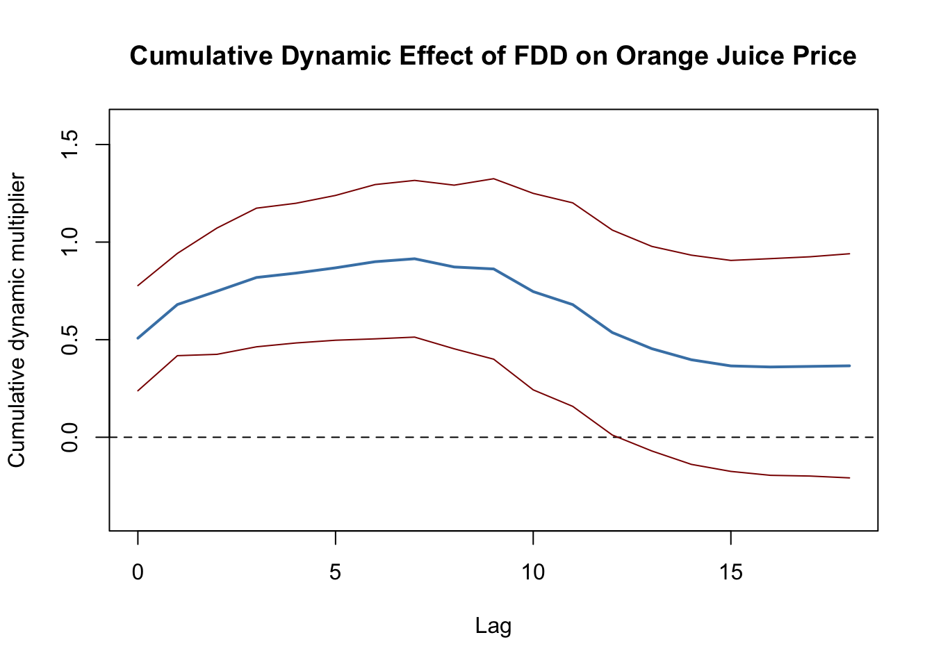
Figure 15.2: Dynamic Cumulative Multipliers
As can be seen from Figure 15.2, the estimated dynamic cumulative multipliers grow until the seventh month up to a price increase of about \(0.91\%\) and then decrease slightly to the estimated long-run cumulative multiplier of \(0.37\%\) which, however, is not significantly different from zero at the \(5\%\) level.
Have the dynamic multipliers been stable over time? One way to see this is to estimate these multipliers for different subperiods of the sample span. For example, consider periods 1950 - 1966, 1967 - 1983 and 1984 - 2000. If the multipliers are the same for all three periods the estimates should be close and thus the estimated cumulative multipliers should be similar, too. We investigate this by re-estimating FOJC_mod_CM1 for the three different time spans and then plot the estimated cumulative dynamic multipliers for the comparison.
# estimate cumulative multiplieres using different sample periods
FOJC_mod_CM1950 <- update(FOJC_mod_CM1, start = c(1950, 1), end = c(1966, 12))

FOJC_mod_CM1967 <- update(FOJC_mod_CM1, start = c(1967, 1), end = c(1983, 12))

FOJC_mod_CM1984 <- update(FOJC_mod_CM1, start = c(1984, 1), end = c(2000, 12))
# plot estimated dynamic cumulative multipliers (1950-1966)
plot(0:18, FOJC_mod_CM1950$coefficients[-1],
type = "l",
lwd = 2,
col = "steelblue",
xlim = c(0, 20),
ylim = c(-0.5, 2),
xlab = "Lag",
ylab = "Cumulative dynamic multiplier",
main = "Cumulative Dynamic Effect for Different Sample Periods")
# plot estimated dynamic multipliers (1967-1983)
lines(0:18, FOJC_mod_CM1967$coefficients[-1], lwd = 2)
# plot estimated dynamic multipliers (1984-2000)
lines(0:18, FOJC_mod_CM1984$coefficients[-1], lwd = 2, col = "darkgreen")
# add dashed line at 0
abline(h = 0, lty = 2)
# add annotations
text(18, -0.24, "1984 - 2000")
text(18, 0.6, "1967 - 1983")
text(18, 1.2, "1950 - 1966")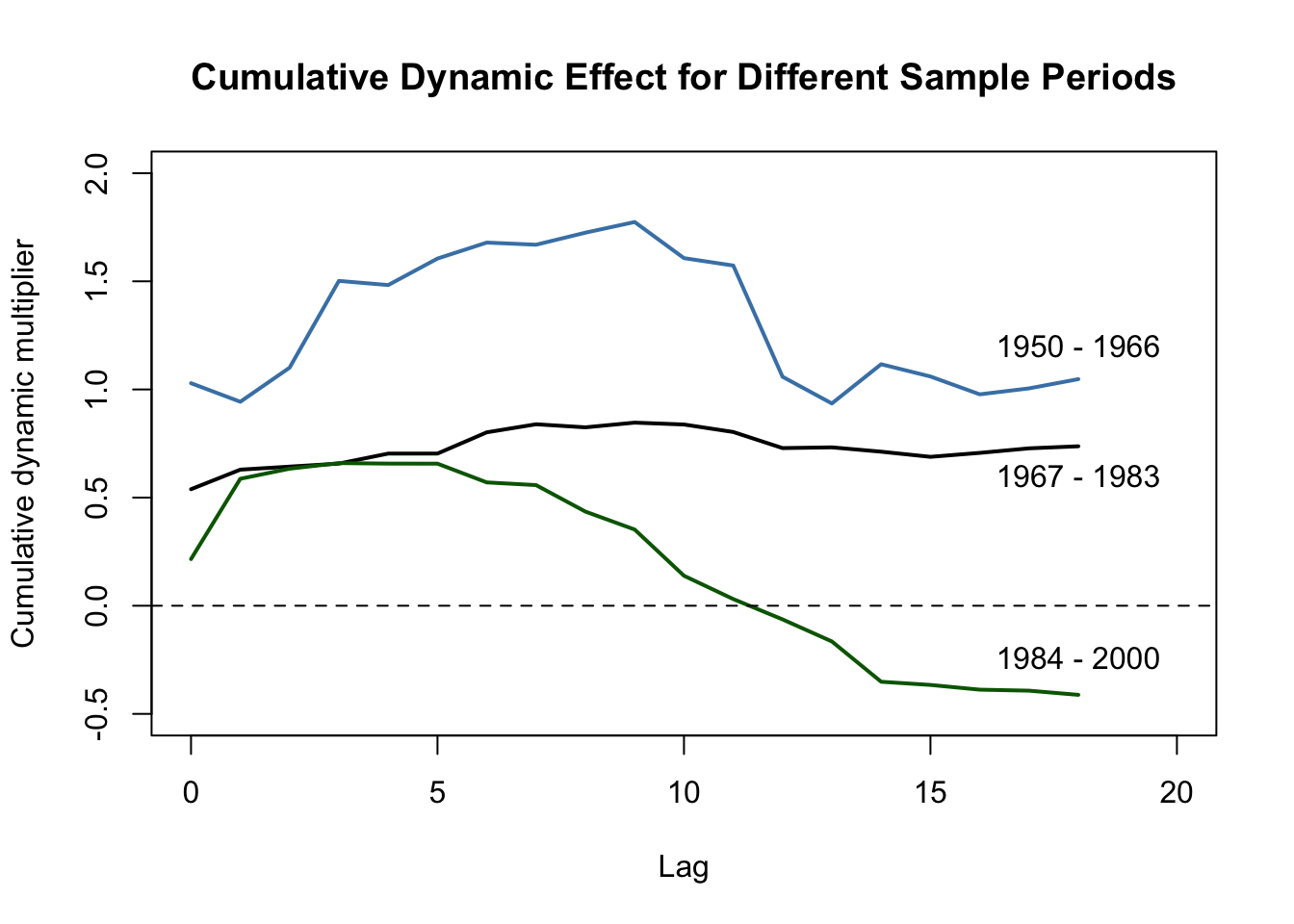
Clearly, the cumulative dynamic multipliers have changed considerably over time. The effect of a freeze was stronger and more persistent in the 1950s and 1960s. For the 1970s the magnitude of the effect was lower but still highly persistent. We observe an even lower magnitude for the final third of the sample span (1984 - 2000) where the long-run effect is much less persistent and essentially zero after a year.
A QLR test for a break in the distributed lag regression of column (1) in Table @ref{tab:deoafddotpooj} with \(15\%\) trimming using a HAC variance-covariance matrix estimate supports the conjecture that the population regression coefficients have changed over time.
# set up a range of possible break dates
tau <- c(window(time(FDD),
                time(FDD)[round(612/100*15)],
                time(FDD)[round(612/100*85)]))

# initialize the vector of F-statistics
Fstats <- numeric(length(tau))

# the restricted model
res_model <- dynlm(FOJC_pctc ~ L(FDD, 0:18))

# estimation, loop over break dates
for(i in 1:length(tau)) {

  # set up dummy variable
  D <- time(FOJC_pctc) > tau[i]

  # estimate DL model with intercations
  unres_model <- dynlm(FOJC_pctc ~ D * L(FDD, 0:18))

  # compute and save F-statistic
  Fstats[i] <- waldtest(res_model,
                        unres_model,
                        vcov = NeweyWest(unres_model, lag = 7, prewhite = F))$F[2]

}
Note that this code takes a couple of seconds to run since a total of length(tau) regressions with \(40\) model coefficients each are estimated.
# QLR test statistic
max(Fstats)
## [1] 36.76819The QLR statistic is \(36.77\). From Table 14.5 of the book we see that the \(1\%\) critical value for the QLR test with \(15\%\) trimming and \(q=20\) restrictions is \(2.43\). Since this is a right-sided test, the QLR statistic clearly lies in the region of rejection so we can discard the null hypothesis of no break in the population regression function.
See Chapter 15.7 of the book for a discussion of empirical examples where it is questionable whether the assumption of (past and present) exogeneity of the regressors is plausible.
Summary
We have seen how R can be used to estimate the time path of the effect on \(Y\) of a change in \(X\) (the dynamic causal effect on \(Y\) of a change in \(X\)) using time series data on both. The corresponding model is called the distributed lag model. Distributed lag models are conveniently estimated using the function dynlm() from the package dynlm.
The regression error in distributed lag models is often serially correlated such that standard errors which are robust to heteroskedasticity and autocorrelation should be used to obtain valid inference. The package sandwich provides functions for computation of so-called HAC covariance matrix estimators, for example vcovHAC() and NeweyWest().
When \(X\) is strictly exogeneous, more efficient estimates can be obtained using an ADL model or by GLS estimation. Feasible GLS algorithms can be found in the R packages orcutt and nlme. Chapter 15.7 of the book emphasizes that the assumption of strict exogeneity is often implausible in empirical applications.