14.9 Can You Beat the Market? (Part II)
The dividend yield (the ratio of current dividends to the stock price) can be considered as an indicator of future dividends: if a stock has a high current dividend yield, it can be considered undervalued and it can be presumed that the price of the stock goes up in the future, meaning that future excess returns go up.
This presumption can be examined using ADL models of excess returns, where lags of the logarithm of the stock’s dividend yield serve as additional regressors.
Unfortunately, a graphical inspection of the time series of the logarithm of the dividend yield casts doubt on the assumption that the series is stationary which, as has been discussed in Chapter 14.7, is necessary to conduct standard inference in a regression analysis.
# plot logarithm of dividend yield series
plot(StockReturns[, 2],
     col = "steelblue",
     lwd = 2,
     ylab = "Logarithm",
     main = "Dividend Yield for CRSP Index")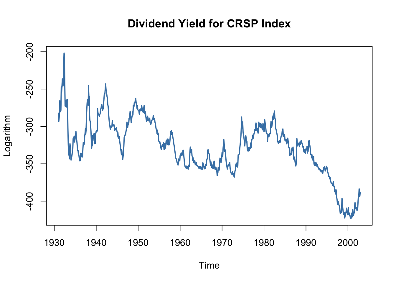
The Dickey-Fuller test statistic for an autoregressive unit root in an AR(\(1\)) model with drift provides further evidence that the series might be nonstationary.
# test for unit root in GDP using 'ur.df()' from the package 'urca'
summary(ur.df(window(StockReturns[, 2],
                     c(1960,1),
                     c(2002, 12)),
              type = "drift",
              lags = 0))
##
## ###############################################
## # Augmented Dickey-Fuller Test Unit Root Test #
## ###############################################
##
## Test regression drift
##
##
## Call:
## lm(formula = z.diff ~ z.lag.1 + 1)
##
## Residuals:
## Min 1Q Median 3Q Max
## -14.3540 -2.9118 -0.2952 2.6374 25.5170
##
## Coefficients:
## Estimate Std. Error t value Pr(>|t|)
## (Intercept) -2.740964 2.080039 -1.318 0.188
## z.lag.1 -0.007652 0.005989 -1.278 0.202
##
## Residual standard error: 4.45 on 513 degrees of freedom
## Multiple R-squared: 0.003172, Adjusted R-squared: 0.001229
## F-statistic: 1.633 on 1 and 513 DF, p-value: 0.2019
##
##
## Value of test-statistic is: -1.2777 0.9339
##
## Critical values for test statistics:
## 1pct 5pct 10pct
## tau2 -3.43 -2.86 -2.57
## phi1 6.43 4.59 3.78We use window() to get observations from January 1960 to December 2012 only.
Since the \(t\)-value for the coefficient on the lagged logarithm of the dividend yield is \(-1.27\), the hypothesis that the true coefficient is zero cannot be rejected, even at the \(10\%\) significance level.
However, it is possible to examine whether the dividend yield has predictive power for excess returns by using its differences in an ADL(\(1\),\(1\)) and an ADL(\(2\),\(2\)) model (remember that differencing a series with a unit root yields a stationary series), although these model specifications do not correspond to the economic reasoning mentioned above. Thus, we also estimate an ADL(\(1\),\(1\)) regression using the level of the logarithm of the dividend yield.
That is we estimate three different specifications:
\[\begin{align*} excess \, returns_t =& \, \beta_0 + \beta_1 excess \, returns_{t-1} + \beta_3 \Delta \log(dividend yield_{t-1}) + u_t \\ \\ excess \, returns_t =& \, \beta_0 + \beta_1 excess \, returns_{t-1} + \beta_2 excess \, returns_{t-2} \\ &+ \, \beta_3 \Delta \log(dividend yield_{t-1}) + \beta_4 \Delta \log(dividend yield_{t-2}) + u_t \\ \\ excess \, returns_t =& \, \beta_0 + \beta_1 excess \, returns_{t-1} + \beta_5 \log(dividend yield_{t-1}) + u_t \\ \end{align*}\]# ADL(1,1) (1st difference of log dividend yield)
CRSP_ADL_1 <- dynlm(ExReturn ~ L(ExReturn) + d(L(ln_DivYield)),
data = StockReturns,
start = c(1960, 1), end = c(2002, 12))
# ADL(2,2) (1st & 2nd differences of log dividend yield)
CRSP_ADL_2 <- dynlm(ExReturn ~ L(ExReturn) + L(ExReturn, 2)
+ d(L(ln_DivYield)) + d(L(ln_DivYield, 2)),
data = StockReturns,
start = c(1960, 1), end = c(2002, 12))
# ADL(1,1) (level of log dividend yield)
CRSP_ADL_3 <- dynlm(ExReturn ~ L(ExReturn) + L(ln_DivYield),
data = StockReturns,
start = c(1960, 1), end = c(1992, 12))# gather robust standard errors
rob_se_CRSP_ADL <- list(sqrt(diag(sandwich(CRSP_ADL_1))),
sqrt(diag(sandwich(CRSP_ADL_2))),
sqrt(diag(sandwich(CRSP_ADL_3))))A tabular representation of the results can then be generated using stargazer().
stargazer(CRSP_ADL_1, CRSP_ADL_2, CRSP_ADL_3,
  title = "ADL Models of Monthly Excess Stock Returns",
  header = FALSE,
  type = "latex",
  column.sep.width = "-5pt",
  no.space = T,
  digits = 3,
  column.labels = c("ADL(1,1)", "ADL(2,2)", "ADL(1,1)"),
  dep.var.caption  = "Dependent Variable: Excess returns on the CSRP value-weighted index",
  dep.var.labels.include = FALSE,
  covariate.labels = c("$excess return_{t-1}$",
                       "$excess return_{t-2}$",
                       "$1^{st} diff log(dividend yield_{t-1})$",
                       "$1^{st} diff log(dividend yield_{t-2})$",
                       "$log(dividend yield_{t-1})$",
                       "Constant"),
se = rob_se_CRSP_ADL) | Dependent Variable: Excess Returns on the CSRP Value-Weighted Index | |||
| ADL(1,1) | ADL(2,2) | ADL(1,1) | |
| (1) | (2) | (3) | |
| excess returnt-1 | 0.059 | 0.042 | 0.078 |
| (0.158) | (0.162) | (0.057) | |
| excess returnt-2 | -0.213 | ||
| (0.193) | |||
| 1st diff log(dividend yieldt-1) | 0.009 | -0.012 | |
| (0.157) | (0.163) | ||
| 1st diff log(dividend yieldt-2) | -0.161 | ||
| (0.185) | |||
| log(dividend yieldt-1) | 0.026** | ||
| (0.012) | |||
| Constant | 0.309 | 0.372* | 8.987** |
| (0.199) | (0.208) | (3.912) | |
| Observations | 516 | 516 | 396 |
| R2 | 0.003 | 0.007 | 0.018 |
| Adjusted R2 | -0.001 | -0.001 | 0.013 |
| Residual Std. Error | 4.338 (df = 513) | 4.337 (df = 511) | 4.407 (df = 393) |
| F Statistic | 0.653 (df = 2; 513) | 0.897 (df = 4; 511) | 3.683** (df = 2; 393) |
| Note: | *p<0.1; **p<0.05; ***p<0.01 | ||
Table 14.3: ADL Models of Monthly Excess Stock Returns
For models (1) and (2) none of the individual \(t\)-statistics suggest that the coefficients are different from zero. Also, we cannot reject the hypothesis that none of the lags have predictive power for excess returns at any common level of significance (an \(F\)-test that the lags have predictive power does not reject for both models).
Things are different for model (3). The coefficient on the level of the logarithm of the dividend yield is different from zero at the \(5\%\) level and the \(F\)-test rejects, too. But we should be suspicious: the high degree of persistence in the dividend yield series probably renders this inference dubious because \(t\)- and \(F\)-statistics may follow distributions that deviate considerably from their theoretical large-sample distributions such that the usual critical values cannot be applied.
If model (3) were of use for predicting excess returns, pseudo-out-of-sample forecasts based on (3) should at least outperform forecasts of an intercept-only model in terms of the sample RMSFE. We can perform this type of comparison using R code in the fashion of the applications of Chapter 14.8.
# end of sample dates
EndOfSample <- as.numeric(window(time(StockReturns), c(1992, 12), c(2002, 11)))

# initialize matrix  forecasts
forecasts <- matrix(nrow = 2,
                    ncol = length(EndOfSample))

# estimation loop over end of sample dates
for(i in 1:length(EndOfSample)) {

  # estimate model (3)
  mod3 <- dynlm(ExReturn ~ L(ExReturn) + L(ln_DivYield), data = StockReturns,
                start = c(1960, 1),
                end = EndOfSample[i])

  # estimate intercept only model
  modconst <- dynlm(ExReturn ~ 1, data = StockReturns,
                start = c(1960, 1),
                end = EndOfSample[i])

  # sample data for one-period ahead forecast
  t <- window(StockReturns, EndOfSample[i], EndOfSample[i])

  # compute forecast
  forecasts[, i] <- c(coef(mod3) %*% c(1, t[1], t[2]), coef(modconst))

}
# gather data
d <- cbind("Excess Returns" = c(window(StockReturns[,1], c(1993, 1), c(2002, 12))),
"Model (3)" = forecasts[1,],
"Intercept Only" = forecasts[2,],
"Always Zero" = 0)
# Compute RMSFEs
c("ADL model (3)" = sd(d[, 1] - d[, 2]),
"Intercept-only model" = sd(d[, 1] - d[, 3]),
"Always zero" = sd(d[,1] - d[, 4]))## ADL model (3) Intercept-only model Always zero
## 4.043757 4.000221 3.995428The comparison indicates that model (3) is not useful since it is outperformed in terms of sample RMSFE by the intercept-only model. A model forecasting excess returns always to be zero has an even lower sample RMSFE. This finding is consistent with the weak-form efficiency hypothesis which states that all publicly available information is accounted for in stock prices such that there is no way to predict future stock prices or excess returns using past observations, implying that the perceived significant relationship indicated by model (3) is wrong.
Summary
This chapter dealt with introductory topics in time series regression analysis, where variables are generally correlated from one observation to the next, a concept termed serial correlation. We presented several ways of storing and plotting time series data using R and used these for informal analysis of economic data.
We have introduced AR and ADL models and applied them in the context of forecasting of macroeconomic and financial time series using R. The discussion also included the topic of lag length selection. It was shown how to set up a simple function that computes the BIC for a model object supplied.
We have also seen how to write simple R code for performing and evaluating forecasts and demonstrated some more sophisticated approaches to conduct pseudo-out-of-sample forecasts for assessment of a model’s predictive power for unobserved future outcomes of a series, to check model stability and to compare different models.
Furthermore, some more technical aspects like the concept of stationarity were addressed. This included applications to testing for an autoregressive unit root with the Dickey-Fuller test and the detection of a break in the population regression function using the \(QLR\) statistic. For both methods, the distribution of the relevant test statistic is non-normal, even in large samples. Concerning the Dickey-Fuller test we have used R’s random number generation facilities to produce evidence for this by means of a Monte-Carlo simulation and motivated usage of the quantiles tabulated in the book.
Also, empirical studies regarding the validity of the weak and the strong form efficiency hypothesis which are presented in the applications Can You Beat the Market? Part I & II in the book have been reproduced using R.
In all applications of this chapter, the focus was on forecasting future outcomes rather than estimation of causal relationships between time series variables. However, the methods needed for the latter are quite similar. Chapter 15 is devoted to estimation of so called dynamic causal effects.