1.1 A Very Short Introduction to R and RStudio
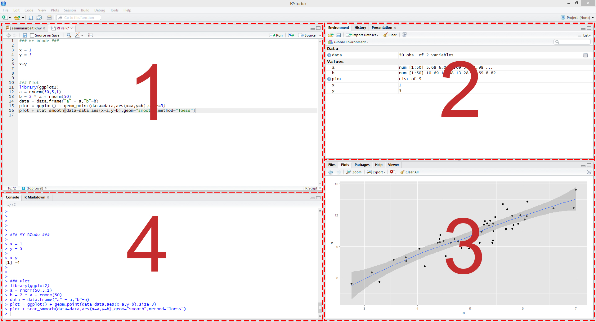
Figure 1.1: RStudio: the four panes
R Basics
As mentioned before, this book is not intended to be an introduction to R but as a guide on how to use its capabilities for applications commonly encountered in undergraduate econometrics. Those having basic knowledge in R programming will feel comfortable starting with Chapter 2. This section, however, is meant for those who have not worked with R or RStudio before. If you at least know how to create objects and call functions, you can skip it. If you would like to refresh your skills or get a feeling for how to work with RStudio, keep reading.
First of all start RStudio and open a new R script by selecting File, New File, R Script. In the editor pane, type
1 + 1and click on the button labeled Run in the top right corner of the editor. By doing so, your line of code is sent to the console and the result of this operation should be displayed right underneath it. As you can see, R works just like a calculator. You can do all arithmetic calculations by using the corresponding operator (+, -, *, / or ^). If you are not sure what the last operator does, try it out and check the results.
Vectors
R is of course more sophisticated than that. We can work with variables or, more generally, objects. Objects are defined by using the assignment operator <-. To create a variable named x which contains the value 10 type x <- 10 and click the button Run yet again. The new variable should have appeared in the environment pane on the top right. The console however did not show any results, because our line of code did not contain any call that creates output. When you now type x in the console and hit return, you ask R to show you the value of x and the corresponding value should be printed in the console.
x is a scalar, a vector of length \(1\). You can easily create longer vectors by using the function c() (c for “concatenate” or “combine”). To create a vector y containing the numbers \(1\) to \(5\) and print it, do the following.
y <- c(1, 2, 3, 4, 5)
y
## [1] 1 2 3 4 5You can also create a vector of letters or words. For now just remember that characters have to be surrounded by quotes, else they will be parsed as object names.
hello <- c("Hello", "World")Here we have created a vector of length 2 containing the words Hello and World.
Do not forget to save your script! To do so, select File, Save.
Functions
You have seen the function c() that can be used to combine objects. In general, all function calls look the same: a function name is always followed by round parentheses. Sometimes, the parentheses include arguments.
Here are two simple examples.
# generate the vector `z`
z <- seq(from = 1, to = 5, by = 1)

# compute the mean of the enries in `z`
mean(x = z)
## [1] 3In the first line we use a function called seq() to create the exact same vector as we did in the previous section, calling it z. The function takes on the arguments from, to and by which should be self-explanatory. The function mean() computes the arithmetic mean of its argument x. Since we pass the vector z as the argument x, the result is 3!
If you are not sure which arguments a function expects, you may consult the function’s documentation. Let’s say we are not sure how the arguments required for seq() work. We then type ?seq in the console. By hitting return the documentation page for that function pops up in the lower right pane of RStudio. In there, the section Arguments holds the information we seek. On the bottom of almost every help page you find examples on how to use the corresponding functions. This is very helpful for beginners and we recommend to look out for those.
Of course, all of the commands presented above also work in interactive widgets throughout the book. You may try them below.