This book is in Open Review. We want your feedback to make the book better for you and other students. You may annotate some text by selecting it with the cursor and then click the on the pop-up menu. You can also see the annotations of others: click the in the upper right hand corner of the page

3.1 Estimation of the Population Mean

Key Concept 3.1

Estimators and Estimates

Estimators are functions of sample data drawn from an unknown population. Estimates are numeric values computed by estimators based on the sample data. Estimators are random variables because they are functions of random data. Estimates are nonrandom numbers.

Think of some economic variable, for example hourly earnings of college graduates, denoted by $Y$. Suppose we are interested in $\mu_Y$ the mean of $Y$. In order to exactly calculate $\mu_Y$ we would have to interview every working graduate in the economy. We simply cannot do this due to time and cost constraints. However, we can draw a random sample of $n$ i.i.d. observations $Y_1, \dots, Y_n$ and estimate $\mu_Y$ using one of the simplest estimators in the sense of Key Concept 3.1 one can think of, that is,

$$\overline{Y} = \frac{1}{n} \sum_{i=1}^n Y_i,$$

the sample mean of $Y$. Then again, we could use an even simpler estimator for $\mu_Y$: the very first observation in the sample, $Y_1$. Is $Y_1$ a good estimator? For now, assume that

$$Y \sim \chi_{12}^2$$

which is not too unreasonable as hourly income is non-negative and we expect many hourly earnings to be in a range of $5€\,$ to $15€$. Moreover, it is common for income distributions to be skewed to the right — a property of the $\chi^2_{12}$ distribution.

# plot the chi_12^2 distribution
curve(dchisq(x, df=12), 
      from = 0, 
      to = 40, 
      ylab = "density", 
      xlab = "hourly earnings in Euro")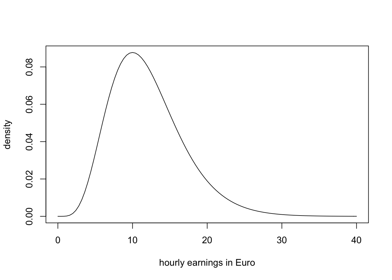Hide Source

Hide Plot

We now draw a sample of $n=100$ observations and take the first observation $Y_1$ as an estimate for $\mu_Y$

# set seed for reproducibility
set.seed(1)

# sample from the chi_12^2 distribution, keep only the first observation
rchisq(n = 100, df = 12)[1]

## [1] 8.257893

The estimate $8.26$ is not too far away from $\mu_Y = 12$ but it is somewhat intuitive that we could do better: the estimator $Y_1$ discards a lot of information and its variance is the population variance:

$$\text{Var}(Y_1) = \text{Var}(Y) = 2 \cdot 12 = 24$$

This brings us to the following question: What is a good estimator of an unknown parameter in the first place? This question is tackled in Key Concepts 3.2 and 3.3.

Key Concept 3.2

Bias, Consistency and Efficiency

Desirable characteristics of an estimator include unbiasedness, consistency and efficiency.

Unbiasedness:
If the mean of the sampling distribution of some estimator $\hat\mu_Y$ for the population mean $\mu_Y$ equals $\mu_Y$, $$E(\hat\mu_Y) = \mu_Y,$$ the estimator is unbiased for $\mu_Y$. The bias of $\hat\mu_Y$ then is $0$:

$$E(\hat\mu_Y) - \mu_Y = 0$$

Consistency:

We want the uncertainty of the estimator $\mu_Y$ to decrease as the number of observations in the sample grows. More precisely, we want the probability that the estimate $\hat\mu_Y$ falls within a small interval around the true value $\mu_Y$ to get increasingly closer to $1$ as $n$ grows. We write this as

$$\hat\mu_Y \xrightarrow{p} \mu_Y.$$

Variance and efficiency:

We want the estimator to be efficient. Suppose we have two estimators, $\hat\mu_Y$ and $\overset{\sim}{\mu}_Y$ and for some given sample size $n$ it holds that

$$E(\hat\mu_Y) = E(\overset{\sim}{\mu}_Y) = \mu_Y$$ but $$\text{Var}(\hat\mu_Y) < \text{Var}(\overset{\sim}{\mu}_Y).$$

We then prefer to use $\hat\mu_Y$ as it has a lower variance than $\overset{\sim}{\mu}_Y$, meaning that $\hat\mu_Y$ is more efficient in using the information provided by the observations in the sample.