5.4 Heteroskedasticity and Homoskedasticity
All inference made in the previous chapters relies on the assumption that the error variance does not vary as regressor values change. But this will often not be the case in empirical applications.
Key Concept 5.4
Heteroskedasticity and Homoskedasticity
The error term of our regression model is homoskedastic if the variance of the conditional distribution of \(u_i\) given \(X_i\), \(Var(u_i|X_i=x)\), is constant for all observations in our sample: \[ \text{Var}(u_i|X_i=x) = \sigma^2 \ \forall \ i=1,\dots,n. \]
If instead there is dependence of the conditional variance of \(u_i\) on \(X_i\), the error term is said to be heteroskedastic. We then write \[ \text{Var}(u_i|X_i=x) = \sigma_i^2 \ \forall \ i=1,\dots,n. \]
- Homoskedasticity is a special case of heteroskedasticity.
For a better understanding of heteroskedasticity, we generate some bivariate heteroskedastic data, estimate a linear regression model and then use box plots to depict the conditional distributions of the residuals.
# load scales package for adjusting color opacities
library(scales)

# generate some heteroskedastic data:

# set seed for reproducibility
set.seed(123)

# set up vector of x coordinates
x <- rep(c(10, 15, 20, 25), each = 25)

# initialize vector of errors
e <- c()

# sample 100 errors such that the variance increases with x
e[1:25] <- rnorm(25, sd = 10)
e[26:50] <- rnorm(25, sd = 15)
e[51:75] <- rnorm(25, sd = 20)
e[76:100] <- rnorm(25, sd = 25)

# set up y
y <- 720 - 3.3 * x + e

# Estimate the model
mod <- lm(y ~ x)

# Plot the data
plot(x = x,
     y = y,
     main = "An Example of Heteroskedasticity",
     xlab = "Student-Teacher Ratio",
     ylab = "Test Score",
     cex = 0.5,
     pch = 19,
     xlim = c(8, 27),
     ylim = c(600, 710))

# Add the regression line to the plot
abline(mod, col = "darkred")

# Add boxplots to the plot
boxplot(formula = y ~ x,
        add = TRUE,
        at = c(10, 15, 20, 25),
        col = alpha("gray", 0.4),
        border = "black"
        )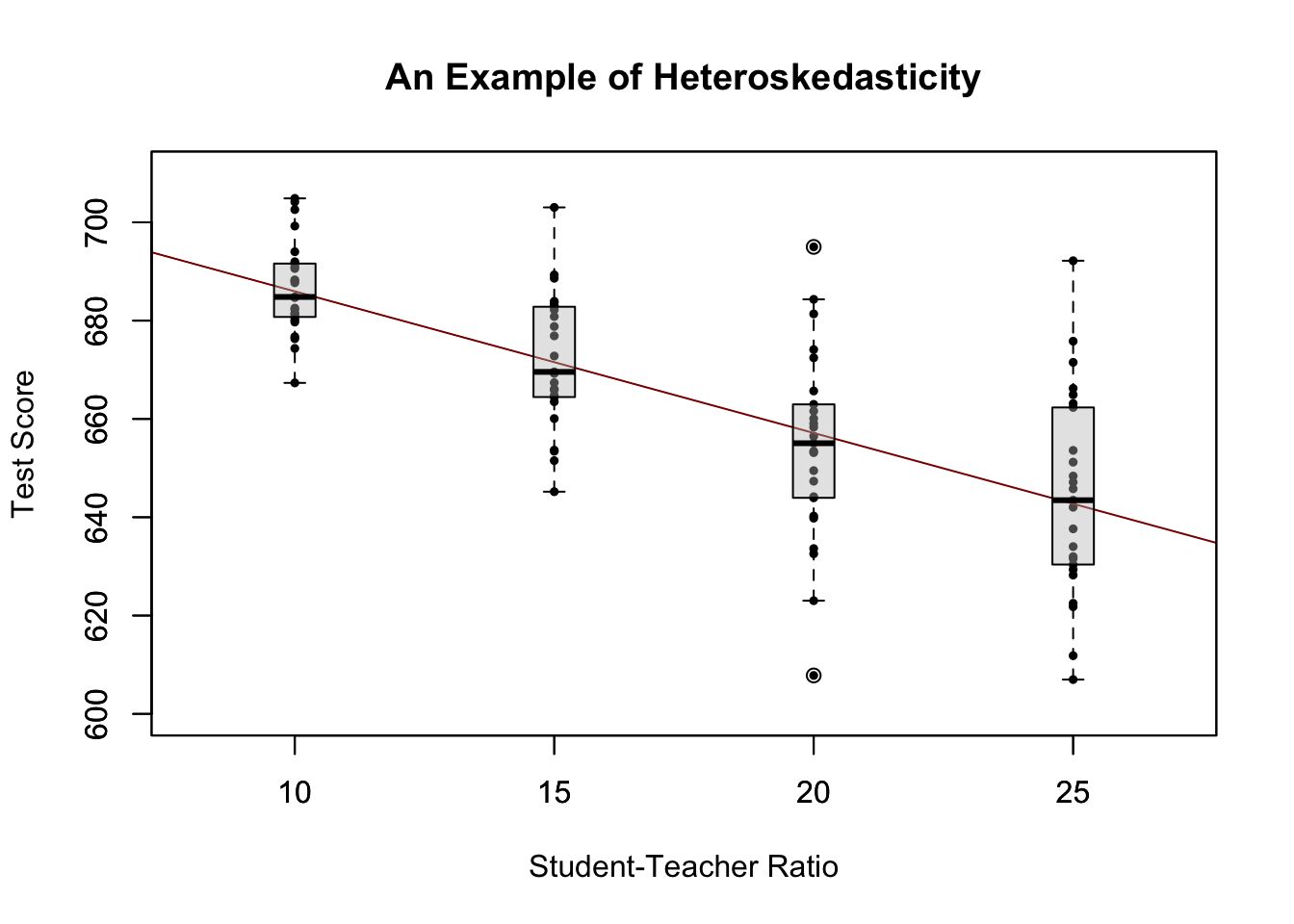
We have used the formula argument y ~ x in boxplot() to specify that we want to split up the vector y into groups according to x. boxplot(y ~ x) generates a boxplot for each of the groups in y defined by x.
For this artificial data it is clear that the conditional error variances differ. Specifically, we observe that the variance in test scores (and therefore the variance of the errors committed) increases with the student teacher ratio.
A Real-World Example for Heteroskedasticity
Think about the economic value of education: if there were no expected economic value-added to receiving university education, you probably would not be reading this script right now. A starting point to empirically verify such a relation is to have data on working individuals. More precisely, we need data on wages and education of workers in order to estimate a model like
\[ wage_i = \beta_0 + \beta_1 \cdot education_i + u_i. \]
What can be presumed about this relation? It is likely that, on average, higher educated workers earn more than workers with less education, so we expect to estimate an upward sloping regression line. Also, it seems plausible that earnings of better educated workers have a higher dispersion then those of low-skilled workers: solid education is not a guarantee for a high salary so even highly qualified workers take on low-income jobs. However, they are more likely to meet the requirements for the well-paid jobs than workers with less education for whom opportunities in the labor market are much more limited.
To verify this empirically we may use real data on hourly earnings and the number of years of education of employees. Such data can be found in CPSSWEducation. This data set is part of the package AER and comes from the Current Population Survey (CPS) which is conducted periodically by the Bureau of Labor Statistics in the United States.
The subsequent code chunks demonstrate how to import the data into R and how to produce a plot in the fashion of Figure 5.3 in the book.
# load package and attach data
library(AER)
data("CPSSWEducation")
attach(CPSSWEducation)

# get an overview
summary(CPSSWEducation)
## age gender earnings education
## Min. :29.0 female:1202 Min. : 2.137 Min. : 6.00
## 1st Qu.:29.0 male :1748 1st Qu.:10.577 1st Qu.:12.00
## Median :29.0 Median :14.615 Median :13.00
## Mean :29.5 Mean :16.743 Mean :13.55
## 3rd Qu.:30.0 3rd Qu.:20.192 3rd Qu.:16.00
## Max. :30.0 Max. :97.500 Max. :18.00# estimate a simple regression model
labor_model <- lm(earnings ~ education)
# plot observations and add the regression line
plot(education,
earnings,
ylim = c(0, 150))
abline(labor_model,
col = "steelblue",
lwd = 2)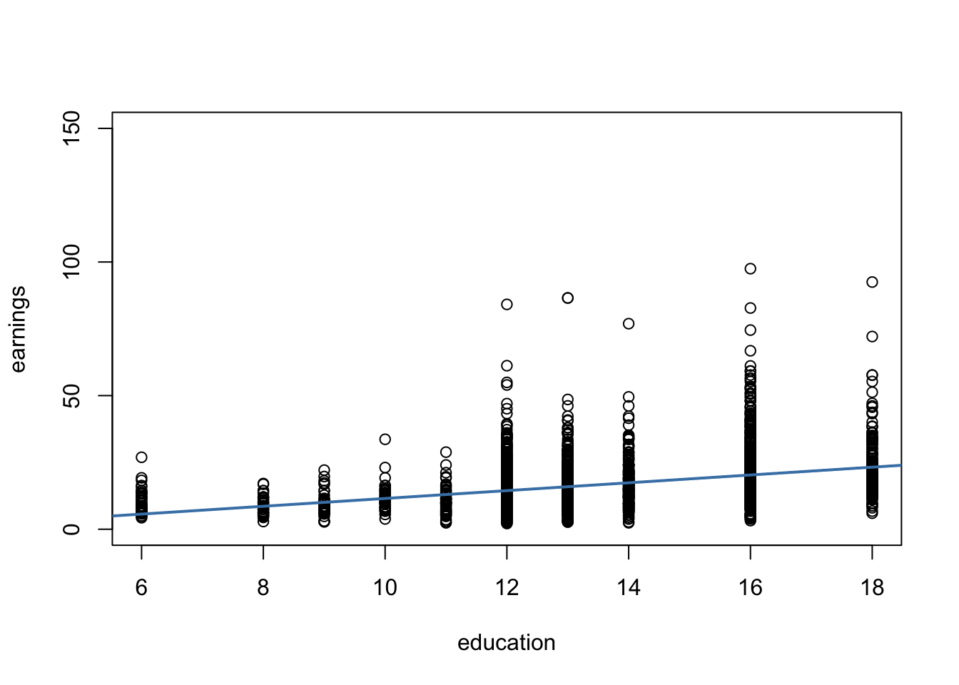
The plot reveals that the mean of the distribution of earnings increases with the level of education. This is also supported by a formal analysis: the estimated regression model stored in labor_mod shows that there is a positive relation between years of education and earnings.
# print the contents of labor_model to the console
labor_model
##
## Call:
## lm(formula = earnings ~ education)
##
## Coefficients:
## (Intercept) education
## -3.134 1.467The estimated regression equation states that, on average, an additional year of education increases a worker’s hourly earnings by about \(\$ 1.47\). Once more we use confint() to obtain a \(95\%\) confidence interval for both regression coefficients.
# compute a 95% confidence interval for the coefficients in the model
confint(labor_model)
## 2.5 % 97.5 %
## (Intercept) -5.015248 -1.253495
## education 1.330098 1.603753Since the interval is \([1.33, 1.60]\) we can reject the hypothesis that the coefficient on education is zero at the \(5\%\) level.
Furthermore, the plot indicates that there is heteroskedasticity: if we assume the regression line to be a reasonably good representation of the conditional mean function \(E(earnings_i\vert education_i)\), the dispersion of hourly earnings around that function clearly increases with the level of education, i.e., the variance of the distribution of earnings increases. In other words: the variance of the errors (the errors made in explaining earnings by education) increases with education so that the regression errors are heteroskedastic.
This example makes a case that the assumption of homoskedasticity is doubtful in economic applications. Should we care about heteroskedasticity? Yes, we should. As explained in the next section, heteroskedasticity can have serious negative consequences in hypothesis testing, if we ignore it.
Should We Care About Heteroskedasticity?
To answer the question whether we should worry about heteroskedasticity being present, consider the variance of \(\hat\beta_1\) under the assumption of homoskedasticity. In this case we have
\[ \sigma^2_{\hat\beta_1} = \frac{\sigma^2_u}{n \cdot \sigma^2_X} \tag{5.5} \]
which is a simplified version of the general equation (4.1) presented in Key Concept 4.4. See Appendix 5.1 of the book for details on the derivation. summary() estimates (5.5) by
\[ \overset{\sim}{\sigma}^2_{\hat\beta_1} = \frac{SER^2}{\sum_{i=1}^n (X_i - \overline{X})^2} \ \ \text{where} \ \ SER=\frac{1}{n-2} \sum_{i=1}^n \hat u_i^2. \]
Thus summary() estimates the homoskedasticity-only standard error
\[ \sqrt{ \overset{\sim}{\sigma}^2_{\hat\beta_1} } = \sqrt{ \frac{SER^2}{\sum_{i=1}^n(X_i - \overline{X})^2} }. \]
This is in fact an estimator for the standard deviation of the estimator \(\hat{\beta}_1\) that is inconsistent for the true value \(\sigma^2_{\hat\beta_1}\) when there is heteroskedasticity. The implication is that \(t\)-statistics computed in the manner of Key Concept 5.1 do not follow a standard normal distribution, even in large samples. This issue may invalidate inference when using the previously treated tools for hypothesis testing: we should be cautious when making statements about the significance of regression coefficients on the basis of \(t\)-statistics as computed by summary() or confidence intervals produced by confint() if it is doubtful for the assumption of homoskedasticity to hold!
We will now use R to compute the homoskedasticity-only standard error for \(\hat{\beta}_1\) in the test score regression model linear_model by hand and see that it matches the value produced by summary().
# Store model summary in 'model'
model <- summary(linear_model)

# Extract the standard error of the regression from model summary
SER <- model$sigma

# Compute the variation in 'size'
V <- (nrow(CASchools)-1) * var(CASchools$STR)

# Compute the standard error of the slope parameter's estimator and print it
SE.beta_1.hat <- sqrt(SER^2/V)
SE.beta_1.hat
## [1] 0.4798255# Use logical operators to see if the value computed by hand matches the one provided
# in mod$coefficients. Round estimates to four decimal places
round(model$coefficients[2, 2], 4) == round(SE.beta_1.hat, 4)## [1] TRUEIndeed, the estimated values are equal.
Computation of Heteroskedasticity-Robust Standard Errors
Consistent estimation of \(\sigma_{\hat{\beta}_1}\) under heteroskedasticity is granted when the following robust estimator is used.
\[ SE(\hat{\beta}_1) = \sqrt{ \frac{1}{n} \cdot \frac{ \frac{1}{n} \sum_{i=1}^n (X_i - \overline{X})^2 \hat{u}_i^2 }{ \left[ \frac{1}{n} \sum_{i=1}^n (X_i - \overline{X})^2 \right]^2} } \tag{5.6} \]
Standard error estimates computed this way are also referred to as Eicker-Huber-White standard errors, the most frequently cited paper on this is White (1980).
It can be quite cumbersome to do this calculation by hand. Luckily, there are R function for that purpose. A convenient one named vcovHC() is part of the package sandwich.6 This function can compute a variety of standard errors. The one brought forward in (5.6) is computed when the argument type is set to “HC0”. Most of the examples presented in the book rely on a slightly different formula which is the default in the statistics package STATA:
\[\begin{align} SE(\hat{\beta}_1)_{HC1} = \sqrt{ \frac{1}{n} \cdot \frac{ \frac{1}{n-2} \sum_{i=1}^n (X_i - \overline{X})^2 \hat{u}_i^2 }{ \left[ \frac{1}{n} \sum_{i=1}^n (X_i - \overline{X})^2 \right]^2}} \tag{5.2} \end{align}\]The difference is that we multiply by \(\frac{1}{n-2}\) in the numerator of (5.2). This is a degrees of freedom correction and was considered by MacKinnon & White (1985). To get vcovHC() to use (5.2), we have to set type = “HC1”.
Let us now compute robust standard error estimates for the coefficients in linear_model.
# compute heteroskedasticity-robust standard errors
vcov <- vcovHC(linear_model, type = "HC1")
vcov
## (Intercept) STR
## (Intercept) 107.419993 -5.3639114
## STR -5.363911 0.2698692The output of vcovHC() is the variance-covariance matrix of coefficient estimates. We are interested in the square root of the diagonal elements of this matrix, i.e., the standard error estimates.
When we have k > 1 regressors, writing down the equations for a regression model becomes very messy. A more convinient way to denote and estimate so-called multiple regression models (see Chapter 6) is by using matrix algebra. This is why functions like vcovHC() produce matrices. In the simple linear regression model, the variances and covariances of the estimators can be gathered in the symmetric variance-covariance matrix
\[\begin{equation} \text{Var} \begin{pmatrix} \hat\beta_0 \\ \hat\beta_1 \end{pmatrix} = \begin{pmatrix} \text{Var}(\hat\beta_0) & \text{Cov}(\hat\beta_0,\hat\beta_1) \\ \text{Cov}(\hat\beta_0,\hat\beta_1) & \text{Var}(\hat\beta_1) \end{pmatrix}, \end{equation}\]so vcovHC() gives us \(\widehat{\text{Var}}(\hat\beta_0)\), \(\widehat{\text{Var}}(\hat\beta_1)\) and \(\widehat{\text{Cov}}(\hat\beta_0,\hat\beta_1)\), but most of the time we are interested in the diagonal elements of the estimated matrix.
# compute the square root of the diagonal elements in vcov
robust_se <- sqrt(diag(vcov))
robust_se
## (Intercept) STR
## 10.3643617 0.5194893Now assume we want to generate a coefficient summary as provided by summary() but with robust standard errors of the coefficient estimators, robust \(t\)-statistics and corresponding \(p\)-values for the regression model linear_model. This can be done using coeftest() from the package lmtest, see ?coeftest. Further we specify in the argument vcov. that vcov, the Eicker-Huber-White estimate of the variance matrix we have computed before, should be used.
# we invoke the function `coeftest()` on our model
coeftest(linear_model, vcov. = vcov)
##
## t test of coefficients:
##
## Estimate Std. Error t value Pr(>|t|)
## (Intercept) 698.93295 10.36436 67.4362 < 2.2e-16 ***
## STR -2.27981 0.51949 -4.3886 1.447e-05 ***
## ---
## Signif. codes: 0 '***' 0.001 '**' 0.01 '*' 0.05 '.' 0.1 ' ' 1We see that the values reported in the column Std. Error are equal those from sqrt(diag(vcov)).
How severe are the implications of using homoskedasticity-only standard errors in the presence of heteroskedasticity? The answer is: it depends. As mentioned above we face the risk of drawing wrong conclusions when conducting significance tests.
Let us illustrate this by generating another example of a heteroskedastic data set and using it to estimate a simple regression model. We take
\[ Y_i = \beta_1 \cdot X_i + u_i \ \ , \ \ u_i \overset{i.i.d.}{\sim} \mathcal{N}(0,0.36 \cdot X_i^2) \]
with \(\beta_1=1\) as the data generating process. Clearly, the assumption of homoskedasticity is violated here since the variance of the errors is a nonlinear, increasing function of \(X_i\) but the errors have zero mean and are i.i.d. such that the assumptions made in Key Concept 4.3 are not violated. As before, we are interested in estimating \(\beta_1\).
# generate heteroskedastic data
X <- 1:500
Y <- rnorm(n = 500, mean = X, sd = 0.6 * X)

# estimate a simple regression model
reg <- lm(Y ~ X)
We plot the data and add the regression line.
# plot the data
plot(x = X, y = Y,
     pch = 19,
     col = "steelblue",
     cex = 0.8)

# add the regression line to the plot
abline(reg,
       col = "darkred",
       lwd = 1.5)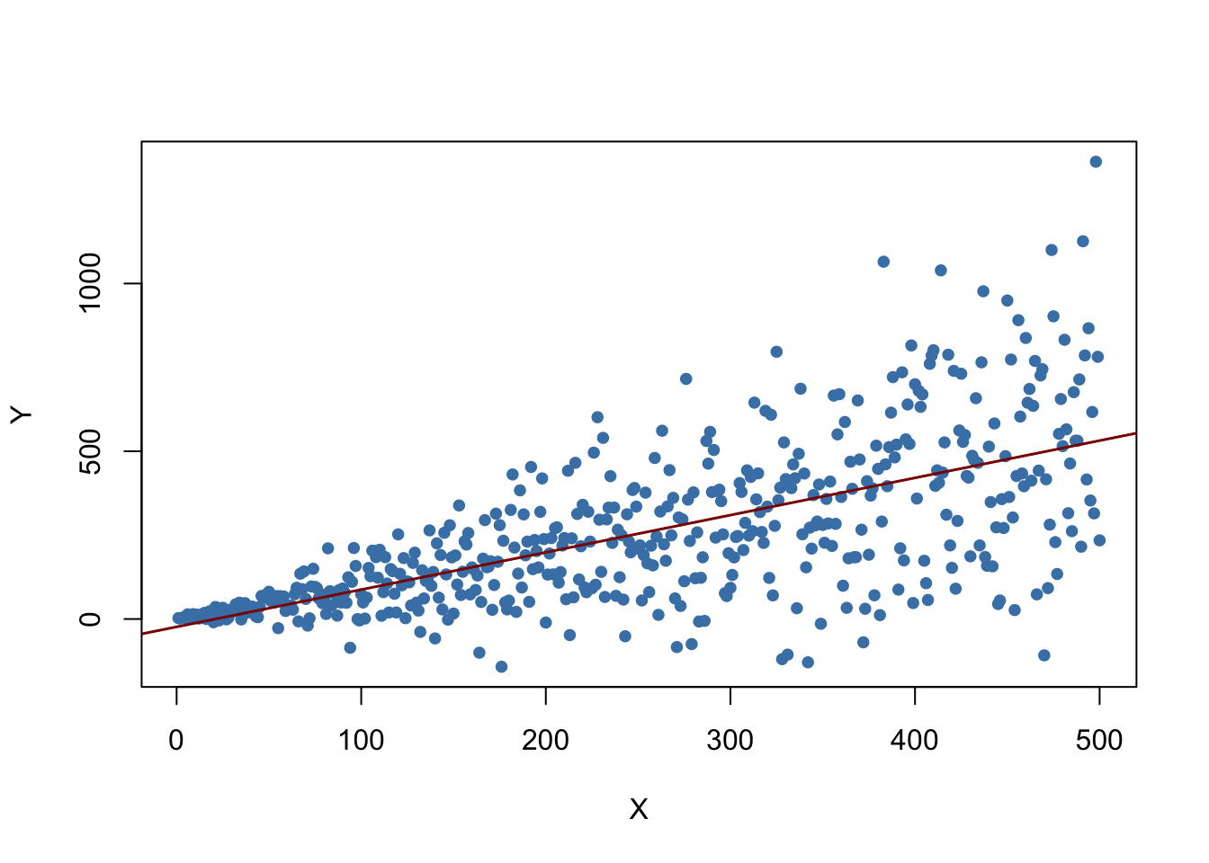
The plot shows that the data are heteroskedastic as the variance of \(Y\) grows with \(X\). We next conduct a significance test of the (true) null hypothesis \(H_0: \beta_1 = 1\) twice, once using the homoskedasticity-only standard error formula and once with the robust version (5.6). An easy way to do this in R is the function linearHypothesis() from the package car, see ?linearHypothesis. It allows to test linear hypotheses about parameters in linear models in a similar way as done with a \(t\)-statistic and offers various robust covariance matrix estimators. We test by comparing the tests’ \(p\)-values to the significance level of \(5\%\).
linearHypothesis() computes a test statistic that follows an \(F\)-distribution under the null hypothesis. We will not loose too much words on the underlying theory. In general, the idea of the \(F\)-test is to compare the fit of different models. When testing a hypothesis about a single coefficient using an \(F\)-test, one can show that the test statistic is simply the square of the corresponding \(t\)-statistic:
\[F = t^2 = \left(\frac{\hat\beta_i - \beta_{i,0}}{SE(\hat\beta_i)}\right)^2 \sim F_{1,n-k-1}\]
In linearHypothesis(), there are different ways to specify the hypothesis to be tested, e.g., using a vector of the type character (as done in the next code chunk), see ?linearHypothesis for alternatives. The function returns an object of class anova which contains further information on the test that can be accessed using the $ operator.# test hypthesis using the default standard error formula
linearHypothesis(reg, hypothesis.matrix = "X = 1")$'Pr(>F)'[2] < 0.05## [1] TRUE# test hypothesis using the robust standard error formula
linearHypothesis(reg, hypothesis.matrix = "X = 1", white.adjust = "hc1")$'Pr(>F)'[2] < 0.05## [1] FALSEThis is a good example of what can go wrong if we ignore heteroskedasticity: for the data set at hand the default method rejects the null hypothesis \(\beta_1 = 1\) although it is true. When using the robust standard error formula the test does not reject the null. Of course, we could this might just be a coincidence and both tests do equally well in maintaining the type I error rate of \(5\%\). This can be further investigated by computing Monte Carlo estimates of the rejection frequencies of both tests on the basis of a large number of random samples. We proceed as follows:
- initialize vectors t and t.rob.
- Using a for() loop, we generate \(10000\) heteroskedastic random samples of size \(1000\), estimate the regression model and check whether the tests falsely reject the null at the level of \(5\%\) using comparison operators. The results are stored in the respective vectors t and t.rob.
- After the simulation, we compute the fraction of false rejections for both tests.
# initialize vectors t and t.rob
t <- c()
t.rob <- c()

# loop sampling and estimation
for (i in 1:10000) {

  # sample data
  X <- 1:1000
  Y <- rnorm(n = 1000, mean = X, sd = 0.6*X)

  # estimate regression model
  reg <- lm(Y ~ X)

  # homoskedasdicity-only significance test
  t[i] <- linearHypothesis(reg, "X = 1")$'Pr(>F)'[2] < 0.05

  # robust significance test
  t.rob[i] <- linearHypothesis(reg, "X = 1", white.adjust = "hc1")$'Pr(>F)'[2] < 0.05

}

# compute the fraction of false rejections
round(cbind(t = mean(t), t.rob = mean(t.rob)), 3)
## t t.rob
## [1,] 0.073 0.05These results reveal the increased risk of falsely rejecting the null using the homoskedasticity-only standard error for the testing problem at hand: with the common standard error estimator, \(7.28\%\) of all tests falsely reject the null hypothesis. In contrast, with the robust test statistic we are closer to the nominal level of \(5\%\).
References
White, H. (1980). A Heteroskedasticity-Consistent Covariance Matrix Estimator and a Direct Test for Heteroskedasticity. Econometrica, 48(4), pp. 817–838.
MacKinnon, J. G., & White, H. (1985). Some heteroskedasticity-consistent covariance matrix estimators with improved finite sample properties. Journal of Econometrics, 29(3), 305–325.
The package sandwich is a dependency of the package AER, meaning that it is attached automatically if you load AER.↩