This book is in Open Review. We want your feedback to make the book better for you and other students. You may annotate some text by selecting it with the cursor and then click the on the pop-up menu. You can also see the annotations of others: click the in the upper right hand corner of the page

5.6 Using the t-Statistic in Regression When the Sample Size Is Small

The three OLS assumptions discussed in Chapter 4 (see Key Concept 4.3) are the foundation for the results on the large sample distribution of the OLS estimators in the simple regression model. What can be said about the distribution of the estimators and their \(t\)-statistics when the sample size is small and the population distribution of the data is unknown? Provided that the three least squares assumptions hold and the errors are normally distributed and homoskedastic (we refer to these conditions as the homoskedastic normal regression assumptions), we have normally distributed estimators and \(t\)-distributed test statistics in small samples.

Recall the definition of a \(t\)-distributed variable

\[ \frac{Z}{\sqrt{W/M}} \sim t_M\]

where \(Z\) is a standard normal random variable, \(W\) is \(\chi^2\) distributed with \(M\) degrees of freedom and \(Z\) and \(W\) are independent. See section 5.6 in the book for a more detailed discussion of the small sample distribution of \(t\)-statistics in regression methods.

Let us simulate the distribution of regression \(t\)-statistics based on a large number of small random samples, say \(n=20\), and compare the simulated distributions to the theoretical distributions which should be \(t_{18}\), the \(t\)-distribution with \(18\) degrees of freedom (recall that \(\text{DF}=n-k-1\)).

# initialize two vectors
beta_0 <- c()
beta_1 <- c()

# loop sampling / estimation / t statistics
for (i in 1:10000) {
  
  X <- runif(20, 0, 20)
  Y <- rnorm(n = 20, mean = X)
  reg <- summary(lm(Y ~ X))
  beta_0[i] <- (reg$coefficients[1, 1] - 0)/(reg$coefficients[1, 2])
  beta_1[i] <- (reg$coefficients[2, 1] - 1)/(reg$coefficients[2, 2])
  
}

# plot the distributions and compare with t_18 density:

# divide plotting area
par(mfrow = c(1, 2))

# plot the simulated density of beta_0
plot(density(beta_0), 
     lwd = 2 , 
     main = expression(widehat(beta)[0]), 
     xlim = c(-4, 4))

# add the t_18 density to the plot
curve(dt(x, df = 18), 
      add = T, 
      col = "red", 
      lwd = 2, 
      lty = 2)

# plot the simulated density of beta_1
plot(density(beta_1), 
     lwd = 2, 
     main = expression(widehat(beta)[1]), xlim = c(-4, 4)
     )

# add the t_18 density to the plot
curve(dt(x, df = 18), 
      add = T, 
      col = "red", 
      lwd = 2, 
      lty = 2)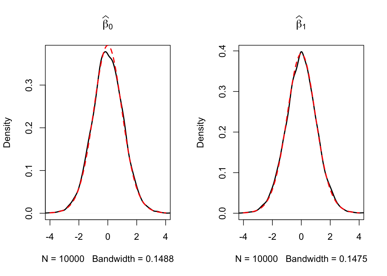 

The outcomes are consistent with our expectations: the empirical distributions of both estimators seem to track the theoretical \(t_{18}\) distribution quite closely.