This book is in Open Review. We want your feedback to make the book better for you and other students. You may annotate some text by selecting it with the cursor and then click the on the pop-up menu. You can also see the annotations of others: click the in the upper right hand corner of the page

6.5 The Distribution of the OLS Estimators in Multiple Regression

As in simple linear regression, different samples will produce different values of the OLS estimators in the multiple regression model. Again, this variation leads to uncertainty of those estimators which we seek to describe using their sampling distribution(s). In short, if the assumption made in Key Concept 6.4 hold, the large sample distribution of $\hat\beta_0,\hat\beta_1,\dots,\hat\beta_k$ is multivariate normal such that the individual estimators themselves are also normally distributed. Key Concept 6.5 summarizes the corresponding statements made in Chapter 6.6 of the book. A more technical derivation of these results can be found in Chapter 18 of the book.

Key Concept 6.5

Large-sample distribution of $\hat\beta_0,\hat\beta_1,\dots,\hat\beta_k$

If the least squares assumptions in the multiple regression model (see Key Concept 6.4) hold, then, in large samples, the OLS estimators $\hat\beta_0,\hat\beta_1,\dots,\hat\beta_k$ are jointly normally distributed. We also say that their joint distribution is multivariate normal. Further, each $\hat\beta_j$ is distributed as $\mathcal{N}(\beta_j,\sigma_{\beta_j}^2)$.

Essentially, Key Concept 6.5 states that, if the sample size is large, we can approximate the individual sampling distributions of the coefficient estimators by specific normal distributions and their joint sampling distribution by a multivariate normal distribution.

How can we use R to get an idea of what the joint PDF of the coefficient estimators in multiple regression model looks like? When estimating a model on some data, we end up with a set of point estimates that do not reveal much information on the joint density of the estimators. However, with a large number of estimations using repeatedly randomly sampled data from the same population we can generate a large set of point estimates that allows us to plot an estimate of the joint density function.

The approach we will use to do this in R is a follows:

• Generate $10000$ random samples of size $50$ using the DGP $$Y_i = 5 + 2.5 \cdot X_{1i} + 3 \cdot X_{2i} + u_i$$ where the regressors $X_{1i}$ and $X_{2i}$ are sampled for each observation as $$X_i = (X_{1i}, X_{2i}) \sim \mathcal{N} \left[\begin{pmatrix} 0 \\ 0 \end{pmatrix}, \begin{pmatrix} 10 & 2.5 \\ 2.5 & 10 \end{pmatrix} \right]$$ and $$u_i \sim \mathcal{N}(0,5)$$ is an error term.

• For each of the $10000$ simulated sets of sample data, we estimate the model $$Y_i = \beta_0 + \beta_1 X_{1i} + \beta_2 X_{2i} + u_i$$ and save the coefficient estimates $\hat\beta_1$ and $\hat\beta_2$.

• We compute a density estimate of the joint distribution of $\hat\beta_1$ and $\hat\beta_2$ in the model above using the function kde2d() from the package MASS, see ?MASS. This estimate is then plotted using the function persp().

# load packages
library(MASS)
library(mvtnorm)

# set sample size
n <- 50

# initialize vector of coefficients
coefs <- cbind("hat_beta_1" = numeric(10000), "hat_beta_2" = numeric(10000))

# set seed for reproducibility
set.seed(1)

# loop sampling and estimation
for (i in 1:10000) {
  
  X <- rmvnorm(n, c(50, 100), sigma = cbind(c(10, 2.5), c(2.5, 10)))
  u <- rnorm(n, sd = 5)
  Y <- 5 + 2.5 * X[, 1] + 3 * X[, 2] + u
  coefs[i,] <- lm(Y ~ X[, 1] + X[, 2])$coefficients[-1]
  
}

# compute density estimate
kde <- kde2d(coefs[, 1], coefs[, 2])

# plot density estimate
persp(kde, 
      theta = 310, 
      phi = 30, 
      xlab = "beta_1", 
      ylab = "beta_2", 
      zlab = "Est. Density")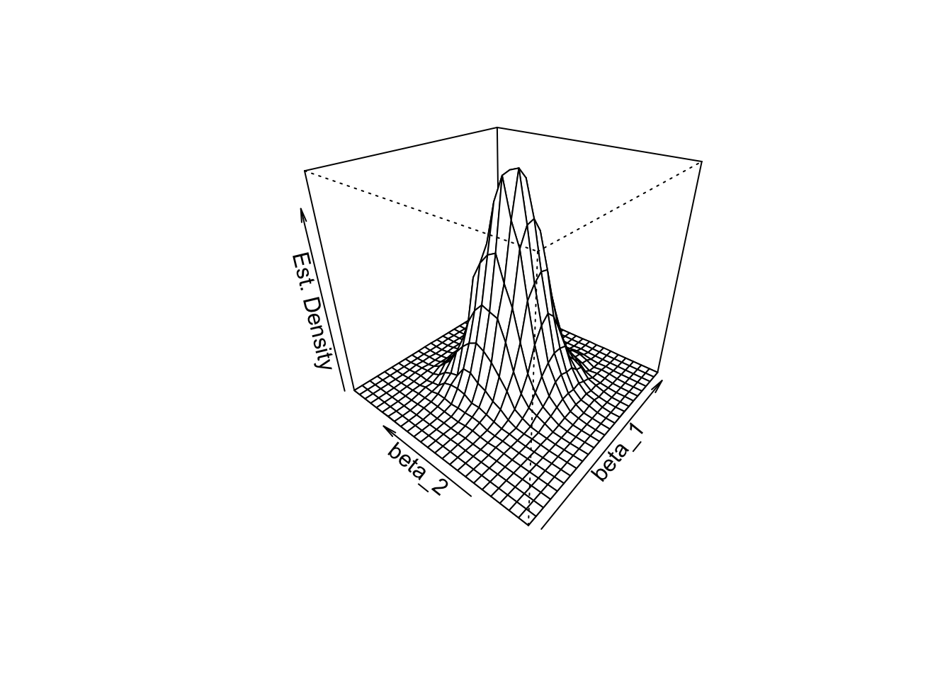

From the plot above we can see that the density estimate has some similarity to a bivariate normal distribution (see Chapter 2) though it is not very pretty and probably a little rough. Furthermore, there is a correlation between the estimates such that $\rho\neq0$ in (2.1). Also, the distribution’s shape deviates from the symmetric bell shape of the bivariate standard normal distribution and has an elliptical surface area instead.

# estimate the correlation between estimators
cor(coefs[, 1], coefs[, 2])

## [1] -0.2503028

Where does this correlation come from? Notice that, due to the way we generated the data, there is correlation between the regressors $X_1$ and $X_2$. Correlation between the regressors in a multiple regression model always translates into correlation between the estimators (see Appendix 6.2 of the book). In our case, the positive correlation between $X_1$ and $X_2$ translates to negative correlation between $\hat\beta_1$ and $\hat\beta_2$. To get a better idea of the distribution you can vary the point of view in the subsequent smooth interactive 3D plot of the same density estimate used for plotting with persp(). Here you can see that the shape of the distribution is somewhat stretched due to $\rho=-0.20$ and it is also apparent that both estimators are unbiased since their joint density seems to be centered close to the true parameter vector $(\beta_1,\beta_2) = (2.5,3)$.