5.2 Confidence Intervals for Regression Coefficients
As we already know, estimates of the regression coefficients \(\beta_0\) and \(\beta_1\) are subject to sampling uncertainty, see Chapter 4. Therefore, we will never exactly estimate the true value of these parameters from sample data in an empirical application. However, we may construct confidence intervals for the intercept and the slope parameter.
A \(95\%\) confidence interval for \(\beta_i\) has two equivalent definitions:
- The interval is the set of values for which a hypothesis test to the level of \(5\%\) cannot be rejected.
- The interval has a probability of \(95\%\) to contain the true value of \(\beta_i\). So in \(95\%\) of all samples that could be drawn, the confidence interval will cover the true value of \(\beta_i\).
We also say that the interval has a confidence level of \(95\%\). The idea of the confidence interval is summarized in Key Concept 5.3.
Key Concept 5.3
A Confidence Interval for \(\beta_i\)
Imagine you could draw all possible random samples of given size. The interval that contains the true value \(\beta_i\) in \(95\%\) of all samples is given by the expression
\[ \text{CI}_{0.95}^{\beta_i} = \left[ \hat{\beta}_i - 1.96 \times SE(\hat{\beta}_i) \, , \, \hat{\beta}_i + 1.96 \times SE(\hat{\beta}_i) \right]. \]
Equivalently, this interval can be seen as the set of null hypotheses for which a \(5\%\) two-sided hypothesis test does not reject.
Simulation Study: Confidence Intervals
To get a better understanding of confidence intervals we conduct another simulation study. For now, assume that we have the following sample of \(n=100\) observations on a single variable \(Y\) where
\[ Y_i \overset{i.i.d}{\sim} \mathcal{N}(5,25), \ i = 1, \dots, 100.\]# set seed for reproducibility
set.seed(4)
# generate and plot the sample data
Y <- rnorm(n = 100,
mean = 5,
sd = 5)
plot(Y,
pch = 19,
col = "steelblue")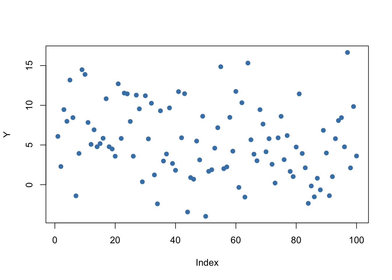
We assume that the data is generated by the model
\[ Y_i = \mu + \epsilon_i \]
where \(\mu\) is an unknown constant and we know that \(\epsilon_i \overset{i.i.d.}{\sim} \mathcal{N}(0,25)\). In this model, the OLS estimator for \(\mu\) is given by \[ \hat\mu = \overline{Y} = \frac{1}{n} \sum_{i=1}^n Y_i, \] i.e., the sample average of the \(Y_i\). It further holds that
\[ SE(\hat\mu) = \frac{\sigma_{\epsilon}}{\sqrt{n}} = \frac{5}{\sqrt{100}} \]
(see Chapter 2) A large-sample \(95\%\) confidence interval for \(\mu\) is then given by
\[\begin{equation} CI^{\mu}_{0.95} = \left[\hat\mu - 1.96 \times \frac{5}{\sqrt{100}} \ , \ \hat\mu + 1.96 \times \frac{5}{\sqrt{100}} \right]. \tag{5.1} \end{equation}\]It is fairly easy to compute this interval in R by hand. The following code chunk generates a named vector containing the interval bounds:
cbind(CIlower = mean(Y) - 1.96 * 5 / 10, CIupper = mean(Y) + 1.96 * 5 / 10)## CIlower CIupper
## [1,] 4.502625 6.462625Knowing that \(\mu = 5\) we see that, for our example data, the confidence interval covers true value.
As opposed to real world examples, we can use R to get a better understanding of confidence intervals by repeatedly sampling data, estimating \(\mu\) and computing the confidence interval for \(\mu\) as in (5.1).
The procedure is as follows:
- We initialize the vectors lower and upper in which the simulated interval limits are to be saved. We want to simulate \(10000\) intervals so both vectors are set to have this length.
- We use a for() loop to sample \(100\) observations from the \(\mathcal{N}(5,25)\) distribution and compute \(\hat\mu\) as well as the boundaries of the confidence interval in every iteration of the loop.
- At last we join lower and upper in a matrix.
# set seed
set.seed(1)

# initialize vectors of lower and upper interval boundaries
lower <- numeric(10000)
upper <- numeric(10000)

# loop sampling / estimation / CI
for(i in 1:10000) {

  Y <- rnorm(100, mean = 5, sd = 5)
  lower[i] <- mean(Y) - 1.96 * 5 / 10
  upper[i] <- mean(Y) + 1.96 * 5 / 10

}

# join vectors of interval bounds in a matrix
CIs <- cbind(lower, upper)
According to Key Concept 5.3 we expect that the fraction of the \(10000\) simulated intervals saved in the matrix CIs that contain the true value \(\mu=5\) should be roughly \(95\%\). We can easily check this using logical operators.
mean(CIs[, 1] <= 5 & 5 <= CIs[, 2])## [1] 0.9487The simulation shows that the fraction of intervals covering \(\mu=5\), i.e., those intervals for which \(H_0: \mu = 5\) cannot be rejected is close to the theoretical value of \(95\%\).
Let us draw a plot of the first \(100\) simulated confidence intervals and indicate those which do not cover the true value of \(\mu\). We do this via horizontal lines representing the confidence intervals on top of each other.
# identify intervals not covering mu
# (4 intervals out of 100)
ID <- which(!(CIs[1:100, 1] <= 5 & 5 <= CIs[1:100, 2]))

# initialize the plot
plot(0,
     xlim = c(3, 7),
     ylim = c(1, 100),
     ylab = "Sample",
     xlab = expression(mu),
     main = "Confidence Intervals")

# set up color vector
colors <- rep(gray(0.6), 100)
colors[ID] <- "red"

# draw reference line at mu=5
abline(v = 5, lty = 2)

# add horizontal bars representing the CIs
for(j in 1:100) {

  lines(c(CIs[j, 1], CIs[j, 2]),
        c(j, j),
        col = colors[j],
        lwd = 2)

}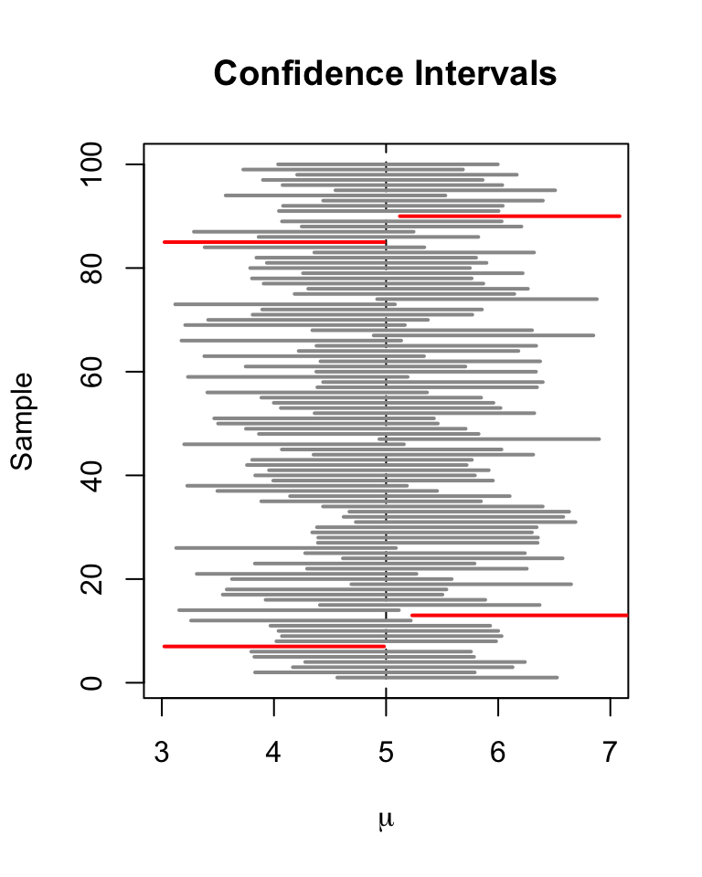
For the first \(100\) samples, the true null hypothesis is rejected in four cases so these intervals do not cover \(\mu=5\). We have indicated the intervals which lead to a rejection of the null red.
Let us now come back to the example of test scores and class sizes. The regression model from Chapter 4 is stored in linear_model. An easy way to get \(95\%\) confidence intervals for \(\beta_0\) and \(\beta_1\), the coefficients on (intercept) and STR, is to use the function confint(). We only have to provide a fitted model object as an input to this function. The confidence level is set to \(95\%\) by default but can be modified by setting the argument level, see ?confint.
# compute 95% confidence interval for coefficients in 'linear_model'
confint(linear_model)
## 2.5 % 97.5 %
## (Intercept) 680.32312 717.542775
## STR -3.22298 -1.336636Let us check if the calculation is done as we expect it to be for \(\beta_1\), the coefficient on STR.
# compute 95% confidence interval for coefficients in 'linear_model' by hand
lm_summ <- summary(linear_model)

c("lower" = lm_summ$coef[2,1] - qt(0.975, df = lm_summ$df[2]) * lm_summ$coef[2, 2],
  "upper" = lm_summ$coef[2,1] + qt(0.975, df = lm_summ$df[2]) * lm_summ$coef[2, 2])
## lower upper
## -3.222980 -1.336636The upper and the lower bounds coincide. We have used the \(0.975\)-quantile of the \(t_{418}\) distribution to get the exact result reported by confint. Obviously, this interval does not contain the value zero which, as we have already seen in the previous section, leads to the rejection of the null hypothesis \(\beta_{1,0} = 0\).