4.5 The Sampling Distribution of the OLS Estimator
Because \(\hat{\beta}_0\) and \(\hat{\beta}_1\) are computed from a sample, the estimators themselves are random variables with a probability distribution — the so-called sampling distribution of the estimators — which describes the values they could take on over different samples. Although the sampling distribution of \(\hat\beta_0\) and \(\hat\beta_1\) can be complicated when the sample size is small and generally changes with the number of observations, \(n\), it is possible, provided the assumptions discussed in the book are valid, to make certain statements about it that hold for all \(n\). In particular \[ E(\hat{\beta}_0) = \beta_0 \ \ \text{and} \ \ E(\hat{\beta}_1) = \beta_1,\] that is, \(\hat\beta_0\) and \(\hat\beta_1\) are unbiased estimators of \(\beta_0\) and \(\beta_1\), the true parameters. If the sample is sufficiently large, by the central limit theorem the joint sampling distribution of the estimators is well approximated by the bivariate normal distribution (2.1). This implies that the marginal distributions are also normal in large samples. Core facts on the large-sample distributions of \(\hat\beta_0\) and \(\hat\beta_1\) are presented in Key Concept 4.4.
Key Concept 4.4
Large Sample Distribution of \(\hat\beta_0\) and \(\hat\beta_1\)
If the least squares assumptions in Key Concept 4.3 hold, then in large samples \(\hat\beta_0\) and \(\hat\beta_1\) have a joint normal sampling distribution. The large sample normal distribution of \(\hat\beta_1\) is \(\mathcal{N}(\beta_1, \sigma^2_{\hat\beta_1})\), where the variance of the distribution, \(\sigma^2_{\hat\beta_1}\), is
\[\begin{align} \sigma^2_{\hat\beta_1} = \frac{1}{n} \frac{Var \left[ \left(X_i - \mu_X \right) u_i \right]} {\left[ Var \left(X_i \right) \right]^2}. \tag{4.1} \end{align}\]The large sample normal distribution of \(\hat\beta_0\) is \(\mathcal{N}(\beta_0, \sigma^2_{\hat\beta_0})\) with
\[\begin{align} \sigma^2_{\hat\beta_0} = \frac{1}{n} \frac{Var \left( H_i u_i \right)}{ \left[ E \left(H_i^2 \right) \right]^2 } \ , \ \text{where} \ \ H_i = 1 - \left[ \frac{\mu_X} {E \left( X_i^2\right)} \right] X_i. \tag{4.2} \end{align}\]The interactive simulation below continuously generates random samples \((X_i,Y_i)\) of \(200\) observations where \(E(Y\vert X) = 100 + 3X\), estimates a simple regression model, stores the estimate of the slope \(\beta_1\) and visualizes the distribution of the \(\widehat{\beta}_1\)s observed so far using a histogram. The idea here is that for a large number of \(\widehat{\beta}_1\)s, the histogram gives a good approximation of the sampling distribution of the estimator. By decreasing the time between two sampling iterations, it becomes clear that the shape of the histogram approaches the characteristic bell shape of a normal distribution centered at the true slope of \(3\).
Simulation Study 1
Whether the statements of Key Concept 4.4 really hold can also be verified using R. For this we first we build our own population of \(100000\) observations in total. To do this we need values for the independent variable \(X\), for the error term \(u\), and for the parameters \(\beta_0\) and \(\beta_1\). With these combined in a simple regression model, we compute the dependent variable \(Y\).
In our example we generate the numbers \(X_i\), \(i = 1\), … ,\(100000\) by drawing a random sample from a uniform distribution on the interval \([0,20]\). The realizations of the error terms \(u_i\) are drawn from a standard normal distribution with parameters \(\mu = 0\) and \(\sigma^2 = 100\) (note that rnorm() requires \(\sigma\) as input for the argument sd, see ?rnorm). Furthermore we chose \(\beta_0 = -2\) and \(\beta_1 = 3.5\) so the true model is
\[ Y_i = -2 + 3.5 \cdot X_i. \]
Finally, we store the results in a data.frame.
# simulate data
N <- 100000
X <- runif(N, min = 0, max = 20)
u <- rnorm(N, sd = 10)

# population regression
Y <- -2 + 3.5 * X + u
population <- data.frame(X, Y)
From now on we will consider the previously generated data as the true population (which of course would be unknown in a real world application, otherwise there would be no reason to draw a random sample in the first place). The knowledge about the true population and the true relationship between \(Y\) and \(X\) can be used to verify the statements made in Key Concept 4.4.
First, let us calculate the true variances \(\sigma^2_{\hat{\beta}_0}\) and \(\sigma^2_{\hat{\beta}_1}\) for a randomly drawn sample of size \(n = 100\).
# set sample size
n <- 100

# compute the variance of beta_hat_0
H_i <- 1 - mean(X) / mean(X^2) * X
var_b0 <- var(H_i * u) / (n * mean(H_i^2)^2 )

# compute the variance of hat_beta_1
var_b1 <- var( ( X - mean(X) ) * u ) / (100 * var(X)^2)
# print variances to the console
var_b0## [1] 4.045066var_b1## [1] 0.03018694Now let us assume that we do not know the true values of \(\beta_0\) and \(\beta_1\) and that it is not possible to observe the whole population. However, we can observe a random sample of \(n\) observations. Then, it would not be possible to compute the true parameters but we could obtain estimates of \(\beta_0\) and \(\beta_1\) from the sample data using OLS. However, we know that these estimates are outcomes of random variables themselves since the observations are randomly sampled from the population. Key Concept 4.4 describes their distributions for large \(n\). When drawing a single sample of size \(n\) it is not possible to make any statement about these distributions. Things change if we repeat the sampling scheme many times and compute the estimates for each sample: using this procedure we simulate outcomes of the respective distributions.
To achieve this in R, we employ the following approach:
- We assign the number of repetitions, say \(10000\), to reps and then initialize a matrix fit were the estimates obtained in each sampling iteration shall be stored row-wise. Thus fit has to be a matrix of dimensions reps\(\times2\).
- In the next step we draw reps random samples of size n from the population and obtain the OLS estimates for each sample. The results are stored as row entries in the outcome matrix fit. This is done using a for() loop.
- At last, we estimate variances of both estimators using the sampled outcomes and plot histograms of the latter. We also add a plot of the density functions belonging to the distributions that follow from Key Concept 4.4. The function bquote() is used to obtain math expressions in the titles and labels of both plots. See ?bquote.
# set repetitions and sample size
n <- 100
reps <- 10000

# initialize the matrix of outcomes
fit <- matrix(ncol = 2, nrow = reps)

# loop sampling and estimation of the coefficients
for (i in 1:reps){

 sample <- population[sample(1:N, n), ]
 fit[i, ] <- lm(Y ~ X, data = sample)$coefficients

}

# compute variance estimates using outcomes
var(fit[, 1])
## [1] 4.057089var(fit[, 2])## [1] 0.03021784# divide plotting area as 1-by-2 array
par(mfrow = c(1, 2))
# plot histograms of beta_0 estimates
hist(fit[, 1],
cex.main = 1,
main = bquote(The ~ Distribution ~ of ~ 10000 ~ beta[0] ~ Estimates),
xlab = bquote(hat(beta)[0]),
freq = F)
# add true distribution to plot
curve(dnorm(x,
-2,
sqrt(var_b0)),
add = T,
col = "darkred")
# plot histograms of beta_hat_1
hist(fit[, 2],
cex.main = 1,
main = bquote(The ~ Distribution ~ of ~ 10000 ~ beta[1] ~ Estimates),
xlab = bquote(hat(beta)[1]),
freq = F)
# add true distribution to plot
curve(dnorm(x,
3.5,
sqrt(var_b1)),
add = T,
col = "darkred")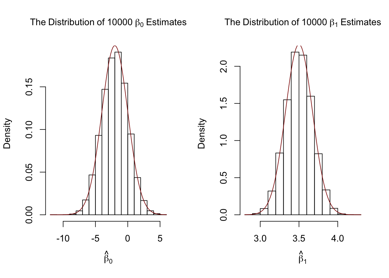
Our variance estimates support the statements made in Key Concept 4.4, coming close to the theoretical values. The histograms suggest that the distributions of the estimators can be well approximated by the respective theoretical normal distributions stated in Key Concept 4.4.
Simulation Study 2
A further result implied by Key Concept 4.4 is that both estimators are consistent, i.e., they converge in probability to the true parameters we are interested in. This is because they are asymptotically unbiased and their variances converge to \(0\) as \(n\) increases. We can check this by repeating the simulation above for a sequence of increasing sample sizes. This means we no longer assign the sample size but a vector of sample sizes: n <- c(…).
Let us look at the distributions of \(\beta_1\). The idea here is to add an additional call of for() to the code. This is done in order to loop over the vector of sample sizes n. For each of the sample sizes we carry out the same simulation as before but plot a density estimate for the outcomes of each iteration over n. Notice that we have to change n to n[j] in the inner loop to ensure that the j\(^{th}\) element of n is used. In the simulation, we use sample sizes of \(100, 250, 1000\) and \(3000\). Consequently we have a total of four distinct simulations using different sample sizes.
# set seed for reproducibility
set.seed(1)

# set repetitions and the vector of sample sizes
reps <- 1000
n <- c(100, 250, 1000, 3000)

# initialize the matrix of outcomes
fit <- matrix(ncol = 2, nrow = reps)

# divide the plot panel in a 2-by-2 array
par(mfrow = c(2, 2))

# loop sampling and plotting

# outer loop over n
for (j in 1:length(n)) {

  # inner loop: sampling and estimating of the coefficients
  for (i in 1:reps){

    sample <- population[sample(1:N, n[j]), ]
    fit[i, ] <- lm(Y ~ X, data = sample)$coefficients

  }

  # draw density estimates
  plot(density(fit[ ,2]), xlim=c(2.5, 4.5),
       col = j,
       main = paste("n=", n[j]),
       xlab = bquote(hat(beta)[1]))

}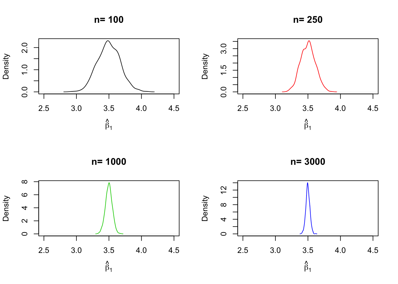
We find that, as \(n\) increases, the distribution of \(\hat\beta_1\) concentrates around its mean, i.e., its variance decreases. Put differently, the likelihood of observing estimates close to the true value of \(\beta_1 = 3.5\) grows as we increase the sample size. The same behavior can be observed if we analyze the distribution of \(\hat\beta_0\) instead.
Simulation Study 3
Furthermore, (4.1) reveals that the variance of the OLS estimator for \(\beta_1\) decreases as the variance of the \(X_i\) increases. In other words, as we increase the amount of information provided by the regressor, that is, increasing \(Var(X)\), which is used to estimate \(\beta_1\), we become more confident that the estimate is close to the true value (i.e., \(Var(\hat\beta_1)\) decreases).
We can visualize this by reproducing Figure 4.6 from the book. To do this, we sample observations \((X_i,Y_i)\), \(i=1,\dots,100\) from a bivariate normal distribution with
\[E(X)=E(Y)=5,\] \[Var(X)=Var(Y)=5\] and \[Cov(X,Y)=4.\]
Formally, this is written down as
\[\begin{align} \begin{pmatrix} X \\ Y \\ \end{pmatrix} \overset{i.i.d.}{\sim} & \ \mathcal{N} \left[ \begin{pmatrix} 5 \\ 5 \\ \end{pmatrix}, \ \begin{pmatrix} 5 & 4 \\ 4 & 5 \\ \end{pmatrix} \right]. \tag{4.3} \end{align}\]To carry out the random sampling, we make use of the function mvrnorm() from the package MASS (Ripley, 2018) which allows to draw random samples from multivariate normal distributions, see ?mvtnorm. Next, we use subset() to split the sample into two subsets such that the first set, set1, consists of observations that fulfill the condition \(\lvert X - \overline{X} \rvert > 1\) and the second set, set2, includes the remainder of the sample. We then plot both sets and use different colors to distinguish the observations.
# load the MASS package
library(MASS)

# set seed for reproducibility
set.seed(4)

# simulate bivarite normal data
bvndata <- mvrnorm(100,
                mu = c(5, 5),
                Sigma = cbind(c(5, 4), c(4, 5)))

# assign column names / convert to data.frame
colnames(bvndata) <- c("X", "Y")
bvndata <- as.data.frame(bvndata)

# subset the data
set1 <- subset(bvndata, abs(mean(X) - X) > 1)
set2 <- subset(bvndata, abs(mean(X) - X) <= 1)

# plot both data sets
plot(set1,
     xlab = "X",
     ylab = "Y",
     pch = 19)

points(set2,
       col = "steelblue",
       pch = 19)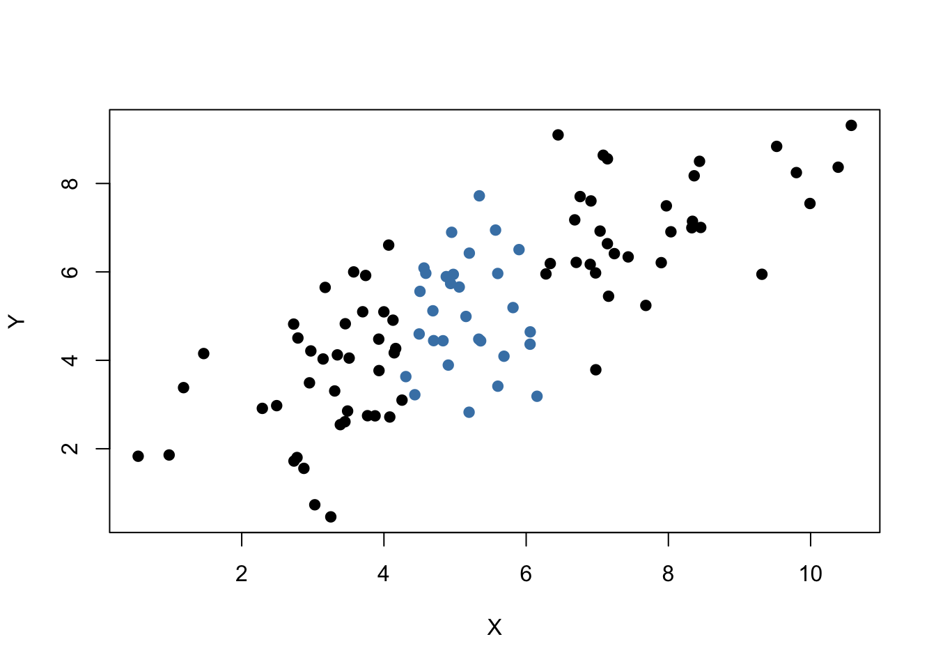
It is clear that observations that are close to the sample average of the \(X_i\) have less variance than those that are farther away. Now, if we were to draw a line as accurately as possible through either of the two sets it is intuitive that choosing the observations indicated by the black dots, i.e., using the set of observations which has larger variance than the blue ones, would result in a more precise line. Now, let us use OLS to estimate slope and intercept for both sets of observations. We then plot the observations along with both regression lines.
# estimate both regression lines
lm.set1 <- lm(Y ~ X, data = set1)
lm.set2 <- lm(Y ~ X, data = set2)

# plot observations
plot(set1, xlab = "X", ylab = "Y", pch = 19)
points(set2, col = "steelblue", pch = 19)

# add both lines to the plot
abline(lm.set1, col = "green")
abline(lm.set2, col = "red")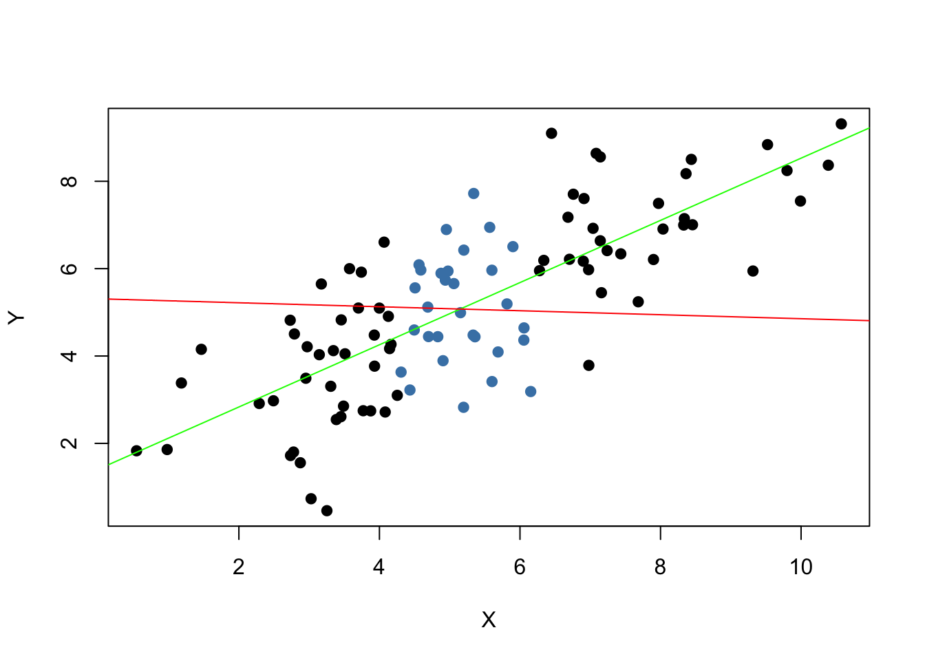
Evidently, the green regression line does far better in describing data sampled from the bivariate normal distribution stated in (4.3) than the red line. This is a nice example for demonstrating why we are interested in a high variance of the regressor \(X\): more variance in the \(X_i\) means more information from which the precision of the estimation benefits.
References
Ripley, B. (2018). MASS: Support Functions and Datasets for Venables and Ripley’s MASS (Version 7.3-50). Retrieved from https://CRAN.R-project.org/package=MASS