Three ways to do it in program R
- Using scalar calculus and algebra (kind of)
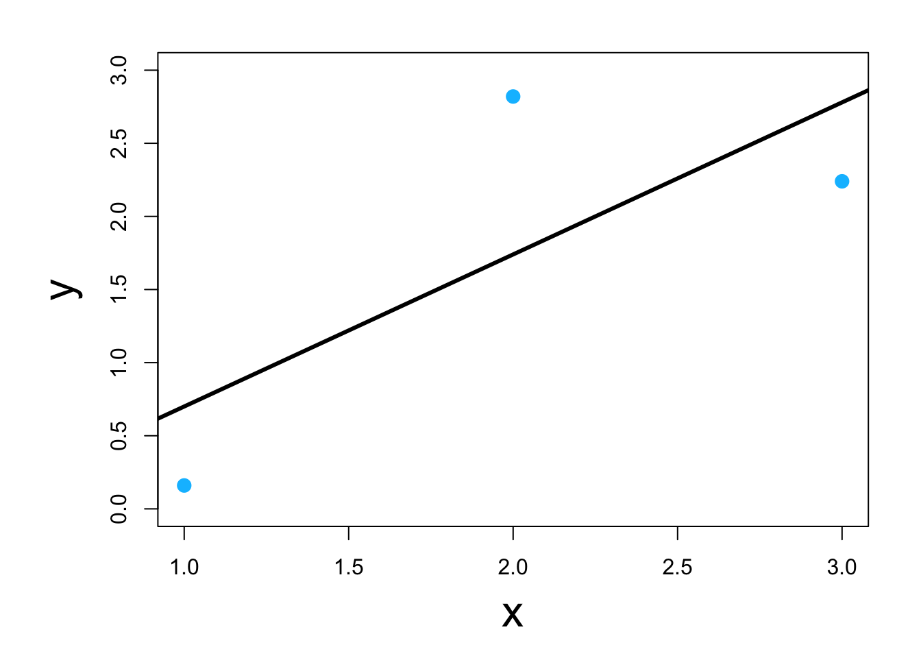
y <- c(0.16,2.82,2.24)
x <- c(1,2,3)

y.bar <- mean(y)
x.bar <- mean(x)

# Estimate the slope parameter
beta1.hat <- sum((x-x.bar)*(y-y.bar))/sum((x-x.bar)^2)
beta1.hat
## [1] 1.04
# Estimate the intercept parameter
beta0.hat <- y.bar - sum((x-x.bar)*(y-y.bar))/sum((x-x.bar)^2)*x.bar
beta0.hat
## [1] -0.34
- Using matrix calculus and algebra
y <- c(0.16,2.82,2.24)
X <- matrix(c(1,1,1,1,2,3),nrow=3,ncol=2,byrow=FALSE)
solve(t(X)%*%X)%*%t(X)%*%y
##       [,1]
## [1,] -0.34
## [2,]  1.04
- Using modern (circa 1970’s) optimization techniques
y <- c(0.16,2.82,2.24)
x <- c(1,2,3)

optim(par=c(0,0),method = c("Nelder-Mead"),fn=function(beta){sum((y-(beta[1]+beta[2]*x))^2)})
## $par
## [1] -0.3399977  1.0399687
##
## $value
## [1] 1.7496
##
## $counts
## function gradient
##       61       NA
##
## $convergence
## [1] 0
##
## $message
## NULL
- Using modern and user friendly statistical computing software
df <- data.frame(y = c(0.16,2.82,2.24),x = c(1,2,3))
lm(y~x,data=df)
##
## Call:
## lm(formula = y ~ x, data = df)
##
## Coefficients:
## (Intercept)            x
##       -0.34         1.04