33 Day 32 (July 22)
33.2 Random effects
Conditional, marginal, and joint distributions
- Conditional distribution: “\(\mathbf{y}\) given \(\boldsymbol{\beta}\)” \[\mathbf{y}|\boldsymbol{\beta}\sim\text{N}(\mathbf{X}\boldsymbol{\beta},\sigma_{\varepsilon}^{2}\mathbf{I})\] This is also sometimes called the data model.
- Marginal distribution of \(\boldsymbol{\beta}\) \[\beta\sim\text{N}(\mathbf{0},\sigma_{\beta}^{2}\mathbf{I})\] This is also called the parameter model.
- Joint distribution \([\mathbf{y}|\boldsymbol{\beta}][\boldsymbol{\beta}]\)
Estimation for the linear model with random effects
- By maximizing the joint likelihood
- Write out the likelihood function \[\mathcal{L}(\boldsymbol{\beta},\sigma_{\varepsilon},\sigma_{\beta}^{2})=\frac{1}{(2\pi)^{-\frac{n}{2}}}|\sigma^{2}_{\varepsilon}\mathbf{I}|^{-\frac{1}{2}}\text{exp}\bigg{(}-\frac{1}{2}(\mathbf{y} - \mathbf{X}\boldsymbol{\beta})^{\prime}(\sigma^{2}_{\varepsilon}\mathbf{I})^{-1}(\mathbf{y} - \mathbf{X}\boldsymbol{\beta})\bigg{)}\times\\\frac{1}{(2\pi)^{-\frac{p}{2}}}|\sigma^{2}_{\beta}\mathbf{I}|^{-\frac{1}{2}}\text{exp}\bigg{(}-\frac{1}{2}\boldsymbol{\beta}^{\prime}(\sigma^{2}_{\beta}\mathbf{I})^{-1}\boldsymbol{\beta}\bigg{)}\]
- Maximizing the log-likelihood function w.r.t. gives \(\boldsymbol{\beta}\) gives \[\hat{\boldsymbol{\beta}}=\big{(}\mathbf{X}^{'}\mathbf{X}+\frac{\sigma^{2}_{\varepsilon}}{\sigma^{2}_{\beta}}\mathbf{I}\big{)}^{-1}\mathbf{X}^{'}\mathbf{y}\]
- By maximizing the joint likelihood
Example eye temperature data set for Eurasian blue tit
df.et <- read.table("https://www.dropbox.com/s/bo11n66cezdnbia/eyetemp.txt?dl=1")
names(df.et) <- c("id","sex","date","time","event","airtemp","relhum","sun","bodycond","eyetemp")
df.et$id <- as.factor(df.et$id)
df.et$id.num <- as.numeric(df.et$id)

ind.means <- aggregate(eyetemp ~ id.num,df.et, FUN=base::mean)
plot(df.et$id.num,df.et$eyetemp,xlab="Individual",ylab="Eye temperature")
points(ind.means,pch="x",col="gold",cex=1.5)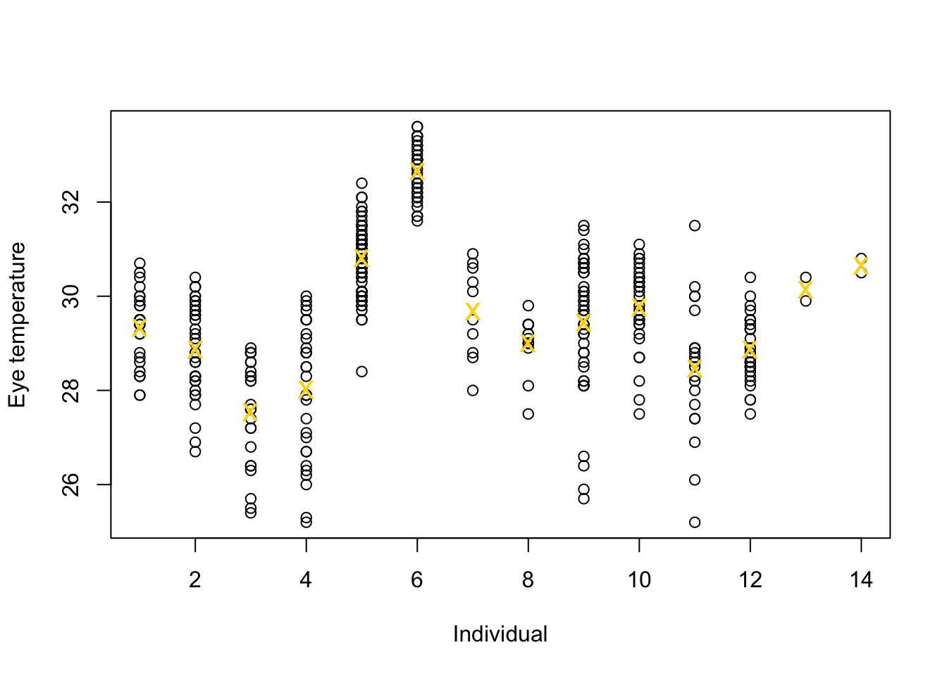
# Standard "fixed effects" linear regression model
m1 <- lm(eyetemp~as.factor(id.num)-1,data=df.et)
summary(m1)
## ## Call: ## lm(formula = eyetemp ~ as.factor(id.num) - 1, data = df.et) ## ## Residuals: ## Min 1Q Median 3Q Max ## -3.7378 -0.5750 0.1507 0.6622 3.0286 ## ## Coefficients: ## Estimate Std. Error t value Pr(>|t|) ## as.factor(id.num)1 29.3423 0.1972 148.77 <2e-16 *** ## as.factor(id.num)2 28.8735 0.1725 167.41 <2e-16 *** ## as.factor(id.num)3 27.5458 0.2053 134.19 <2e-16 *** ## as.factor(id.num)4 28.0156 0.1778 157.59 <2e-16 *** ## as.factor(id.num)5 30.8188 0.1211 254.56 <2e-16 *** ## as.factor(id.num)6 32.6486 0.1700 192.06 <2e-16 *** ## as.factor(id.num)7 29.6800 0.3180 93.33 <2e-16 *** ## as.factor(id.num)8 29.0000 0.2789 103.97 <2e-16 *** ## as.factor(id.num)9 29.4378 0.1499 196.36 <2e-16 *** ## as.factor(id.num)10 29.7667 0.1836 162.12 <2e-16 *** ## as.factor(id.num)11 28.4714 0.2195 129.74 <2e-16 *** ## as.factor(id.num)12 28.8793 0.1867 154.64 <2e-16 *** ## as.factor(id.num)13 30.1500 0.7111 42.40 <2e-16 *** ## as.factor(id.num)14 30.6500 0.7111 43.10 <2e-16 *** ## --- ## Signif. codes: 0 '***' 0.001 '**' 0.01 '*' 0.05 '.' 0.1 ' ' 1 ## ## Residual standard error: 1.006 on 358 degrees of freedom ## Multiple R-squared: 0.9989, Adjusted R-squared: 0.9989 ## F-statistic: 2.31e+04 on 14 and 358 DF, p-value: < 2.2e-16plot(df.et$id.num,df.et$eyetemp,xlab="Individual",ylab="Expected eye temperature",col="white") points(1:14,coef(m1),pch=20,col="black",cex=1) segments (1:14,confint(m1)[,1],1:14,confint(m1)[,2] ,lwd=2,lty=1)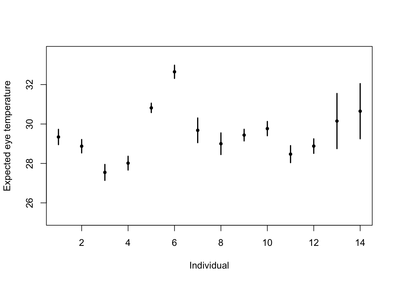
# Random effects regression model (using nlme package; difficult to get confidence interval)
library(nlme)
m2 <- lme(fixed = eyetemp ~ 1,random= list(id = pdIdent(~id-1)),data=df.et,method="ML")#summary(m2)
#predict(m2,level=1,newdata=data.frame(id=unique(df.et$id)))

# Random effects regression model (mgcv package)
library(mgcv)
m2 <- gam(eyetemp ~ 1+s(id,bs="re"),data=df.et,method="ML")

plot(df.et$id.num,df.et$eyetemp,xlab="Individual",ylab="Expected eye temperature",col="white")
points(1:14-0.15,coef(m1),pch=20,col="black",cex=1)
segments (1:14-0.15,confint(m1)[,1],1:14-0.15,confint(m1)[,2] ,lwd=2,lty=1)
pred <- predict(m2,newdata=data.frame(id=unique(df.et$id)),se.fit=TRUE)
pred$lci <- pred$fit - 1.96*pred$se.fit
pred$uci <- pred$fit + 1.96*pred$se.fit
points(1:14+0.15,pred$fit,pch=20,col="green",cex=1)
segments (1:14+0.15,pred$lci,1:14+0.15,pred$uci,lwd=2,lty=1,col="green")
abline(a=coef(m2)[1],b=0,col="grey")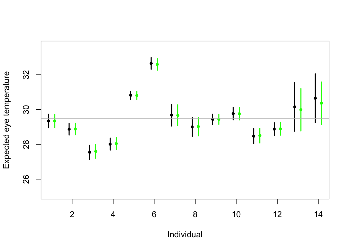
Summary
- Take home message
- Treating \(\boldsymbol{\beta}\) as a random effect “shrinks” the estimates of \(\boldsymbol{\beta}\) closer to zero.
- Requires an extra assumption \(\boldsymbol{\beta}\sim\text{N}(\mathbf{0},\sigma_{\beta}^{2}\mathbf{I})\)
- Penalty
- Random effect
- This called a prior distribution in Bayesian statistics
- Take home message
33.3 Generalized linear models
The generalized linear model framework \[\mathbf{y} \sim[\mathbf{\mathbf{y}|\boldsymbol{\mu},\psi]}\] \[g(\boldsymbol{\mu})=\mathbf{X}\boldsymbol{\beta}\]
- \([\mathbf{y}|\boldsymbol{\mu},\psi]\) is a distribution from the exponential family (e.g., normal, Poisson, binomial) with expected value \(\boldsymbol{\mu}\) and dispersion parameter \(\psi\).
- Example \([\mathbf{y}|\boldsymbol{\mu},\psi]=\text{N}\left(\boldsymbol{\mu},\psi\mathbf{I}\right)\)
- Example \([\mathbf{\mathbf{y}|\boldsymbol{\mu},\psi]}=\text{Poisson}\left(\boldsymbol{\mu}\right)\)
- Example \([\mathbf{\mathbf{y}|\boldsymbol{\mu},\psi]}=\text{gamma}\left(\boldsymbol{\mu},\psi\right)\)
- \([\mathbf{y}|\boldsymbol{\mu},\psi]\) is a distribution from the exponential family (e.g., normal, Poisson, binomial) with expected value \(\boldsymbol{\mu}\) and dispersion parameter \(\psi\).
Estimation
- Use numerical maximization to estimate
- \(\hat{\boldsymbol{\beta}}=(\mathbf{X}^{\prime}\mathbf{X})^{-1}\mathbf{X}^{\prime}\mathbf{y}\) is NOT the MLE for the glm
- Inference is based on asymptotic properties of MLE.
- Example: Challenger data
- The statistical model: \[\mathbf{y}\sim\text{binomial}(6,\mathbf{p})\] \[\text{logit}(\mathbf{p})=\mathbf{X}\boldsymbol{\beta}.\]
- The PMF for the binomial distribution \[\binom{N}{y}p^{y}(1-p)^{N-y}\]
- Write out the likelihood function \[\mathcal{L}(\boldsymbol{\beta})=\prod_{i=1}^n\binom{6}{y_i}p_i^{y_i}(1-p_i)^{6-y_i}\]
- Maximize the log-likelihood function
challenger <- read.csv("https://www.dropbox.com/s/ezxj8d48uh7lzhr/challenger.csv?dl=1")

plot(challenger$Temp,challenger$O.ring,xlab="Temperature",ylab="Number of incidents",xlim=c(10,80),ylim=c(0,6))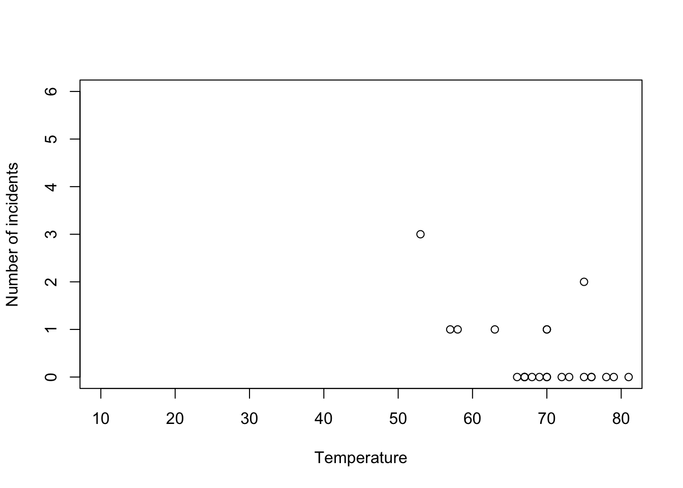
y <- challenger$O.ring
X <- model.matrix(~Temp,data= challenger)

nll <- function(beta){
  p <- 1/(1+exp(-X%*%beta)) # Inverse of logit link function
  -sum(dbinom(y,6,p,log=TRUE)) # Sum of the log likelihood for each observation
  }
est <- optim(par=c(0,0),fn=nll,hessian=TRUE)

# MLE of beta
est$par
## [1] 6.751192 -0.139703## [1] 8.830866682 0.002145791## [1] 2.97167742 0.04632268- Using the
glm()function
m1 <- glm(cbind(challenger$O.ring,6-challenger$O.ring) ~ Temp, family = binomial(link = "logit"),data=challenger)
summary(m1)
## ## Call: ## glm(formula = cbind(challenger$O.ring, 6 - challenger$O.ring) ~ ## Temp, family = binomial(link = "logit"), data = challenger) ## ## Coefficients: ## Estimate Std. Error z value Pr(>|z|) ## (Intercept) 6.75183 2.97989 2.266 0.02346 * ## Temp -0.13971 0.04647 -3.007 0.00264 ** ## --- ## Signif. codes: 0 '***' 0.001 '**' 0.01 '*' 0.05 '.' 0.1 ' ' 1 ## ## (Dispersion parameter for binomial family taken to be 1) ## ## Null deviance: 28.761 on 22 degrees of freedom ## Residual deviance: 19.093 on 21 degrees of freedom ## AIC: 36.757 ## ## Number of Fisher Scoring iterations: 5- Prediction
- We can get prediction using \(\mathbf{X}\hat{\boldsymbol{\beta}}\) or the inverse of the logit link function \(\hat{\boldsymbol{\mu}}=\frac{1}{1+e^{-\mathbf{X}\hat{\boldsymbol{\beta}}}}\)
- Confidence intervals for \(\mathbf{X}\hat{\boldsymbol{\beta}}\) are straightforward
- Confidence intervals for \(\hat{\boldsymbol{\mu}}=\frac{1}{1+e^{-\mathbf{X}\hat{\boldsymbol{\beta}}}}\) are not straightforward because of the nonlinear transformation of \(\hat{\boldsymbol{\beta}}\)
beta.hat <- coef(m1)

new.temp <- seq(0,80,by=0.01)
X.new <- model.matrix(~new.temp)

mu.hat <- (1/(1+exp(-X.new%*%beta.hat)))

plot(challenger$Temp,challenger$O.ring,xlab="Temperature",ylab="Number of incidents",xlim=c(10,80),ylim=c(0,6))
points(new.temp,6*mu.hat,typ="l",col="red")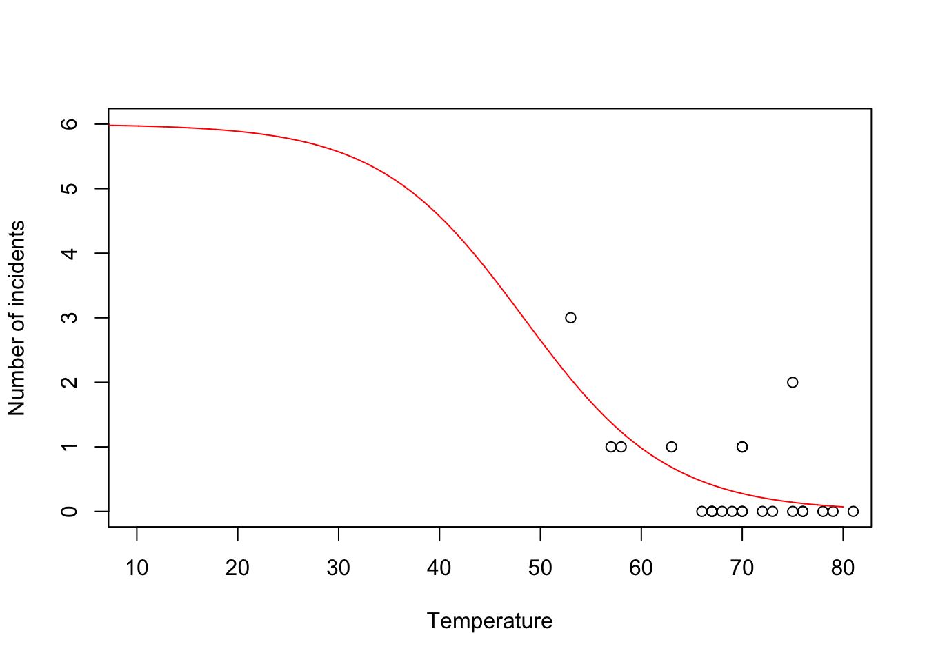
- Predictive distribution
library(mosaic)

predict.bs <- function(){
  m1 <- glm(cbind(O.ring,6-O.ring) ~ Temp, family = binomial(link = "logit"),data=resample(challenger))
  p <- predict(m1,newdata=data.frame(Temp=31),type="response")
  y <- rbinom(1,6,p)
  y
}

bootstrap <- do(1000)*predict.bs()

par(mar = c(5, 4, 7, 2))
hist(bootstrap[,1], col = "grey", xlab = "Year", main = "Empirical distribution of O-ring failures at 31 degrees", freq = FALSE,right=FALSE,breaks=c(-0.5:6.5))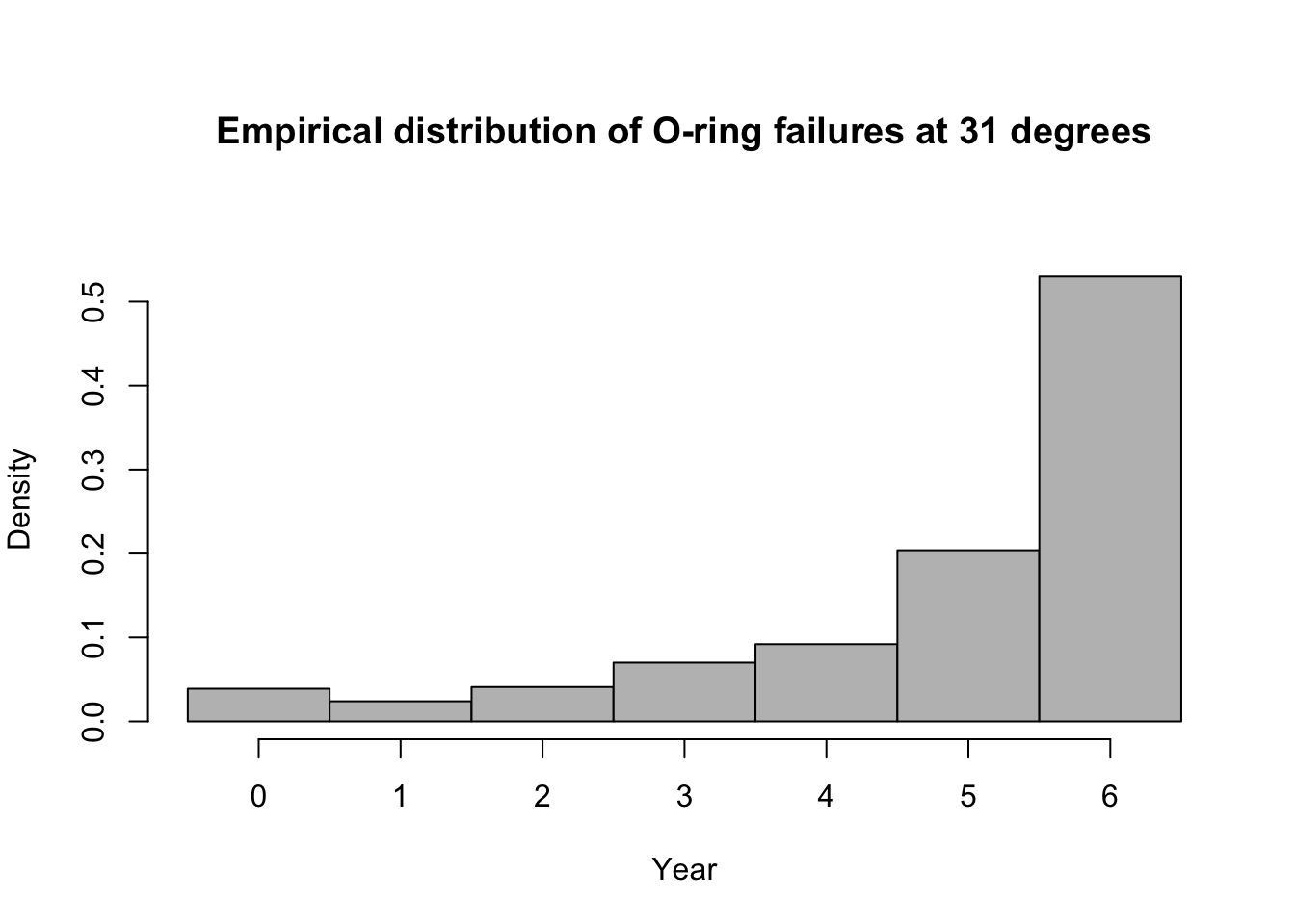
# 95% equal-tailed CI based on percentiles of the empirical distribution
quantile(bootstrap[,1], prob = c(0.025, 0.975))
## 2.5% 97.5% ## 0 6## [1] 0.53Summary
- The generalized linear model useful when the distributional assumptions of linear model are untenable.
- Small counts
- Binary data
- Two cultures
- All distributions are approximations of a unknown data generating process so why does it matter? Use the linear model because it is easier to understand.
- Personal philosophy
- Picking a distribution whose support matches that of the data gets closer to the etiology of the process that generated the data.
- Easier for me to think scientifically about the process
- The generalized linear model useful when the distributional assumptions of linear model are untenable.