42 Assignment 3 (Guide)

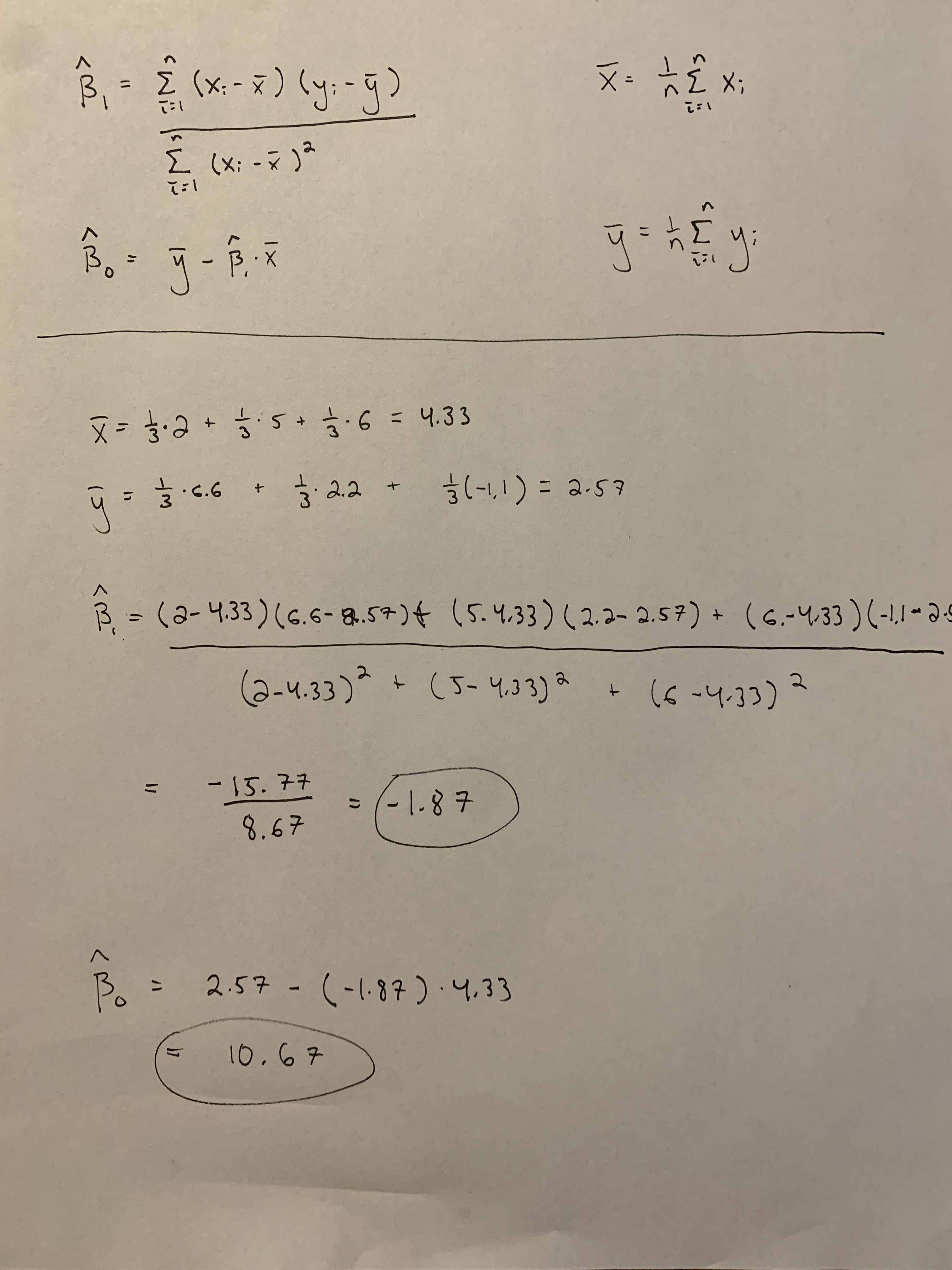
There are multiple ways to calculate the estimates. Below I show how to calculate the estimates using scalars, but you will get the same estimates if you used matrices.
No example answer provided. The question is clear and easy to understand without needing any extra information or explanation. Please re-read the question and make sure you actually completed what was asked (e.g., write a 4-5 sentence description).
A linear model that can be used to determine if the temperature in Manhattan has increased over a long time period using the data from question 2 is\[y_t=\beta_{0}+\beta_{1}t+\varepsilon_t,\]where $y_t$ is the observed (recorded) temperature on day $t$. The day, $t$, is the days elapsed since January 1, 1883 (i.e., the first recorded date in the data set). Here, $t=0,1,2,…47639), however, the observed temperature is not available for only 32,539 of 47,639 days (i.e., there are 14,861 missing days of recorded temperature). The $\beta_{0}$ is the intercept terms, which can be interpreted as the expected temperature on day 0. The $\beta_{1}$ is the slope and can be interpreted as the rate of change in the expected temperature on a daily time scale. Finally, the $\varepsilon_t$ is the error term and accounts for variability in temperature that is not explained by the mathematical part of the model (i.e., $\beta_{0}+\beta_{1}t)$
See R code below. I choose to use the squared error (L2) loss function.

library(lubridate)

## 
## Attaching package: 'lubridate'

## The following objects are masked from 'package:base':
## 
##     date, intersect, setdiff, union

url <- "https://www.dropbox.com/s/asw6gtq7pp1h0bx/manhattan_temp_data.csv?dl=1"
df.temp <- read.csv(url)
df.temp$DATE <- ymd(df.temp$DATE)
df.temp$days <- df.temp$DATE - min(df.temp$DATE)

m1 <- lm(TOBS~days,data=df.temp)
beta0.hat <- coef(m1)[1]
beta1.hat <- coef(m1)[2]
beta0.hat

## (Intercept) 
##    46.42983

beta1.hat

##         days 
## 0.0001902842

Estimates of $\beta_0$ and $\beta_1$ are the same as question 4.

y <- as.numeric(df.temp$TOBS)
x <- as.numeric(df.temp$days)
x <- x[-which(is.na(y)==TRUE)]
y <- y[-which(is.na(y)==TRUE)]

optim(par=c(0,0),method = c("Nelder-Mead"),fn=function(beta){sum(abs(y-(beta[1]+beta[2]*x)))})

## $par
## [1] 4.218326e+01 3.373865e-04
## 
## $value
## [1] 623903.9
## 
## $counts
## function gradient 
##      125       NA 
## 
## $convergence
## [1] 0
## 
## $message
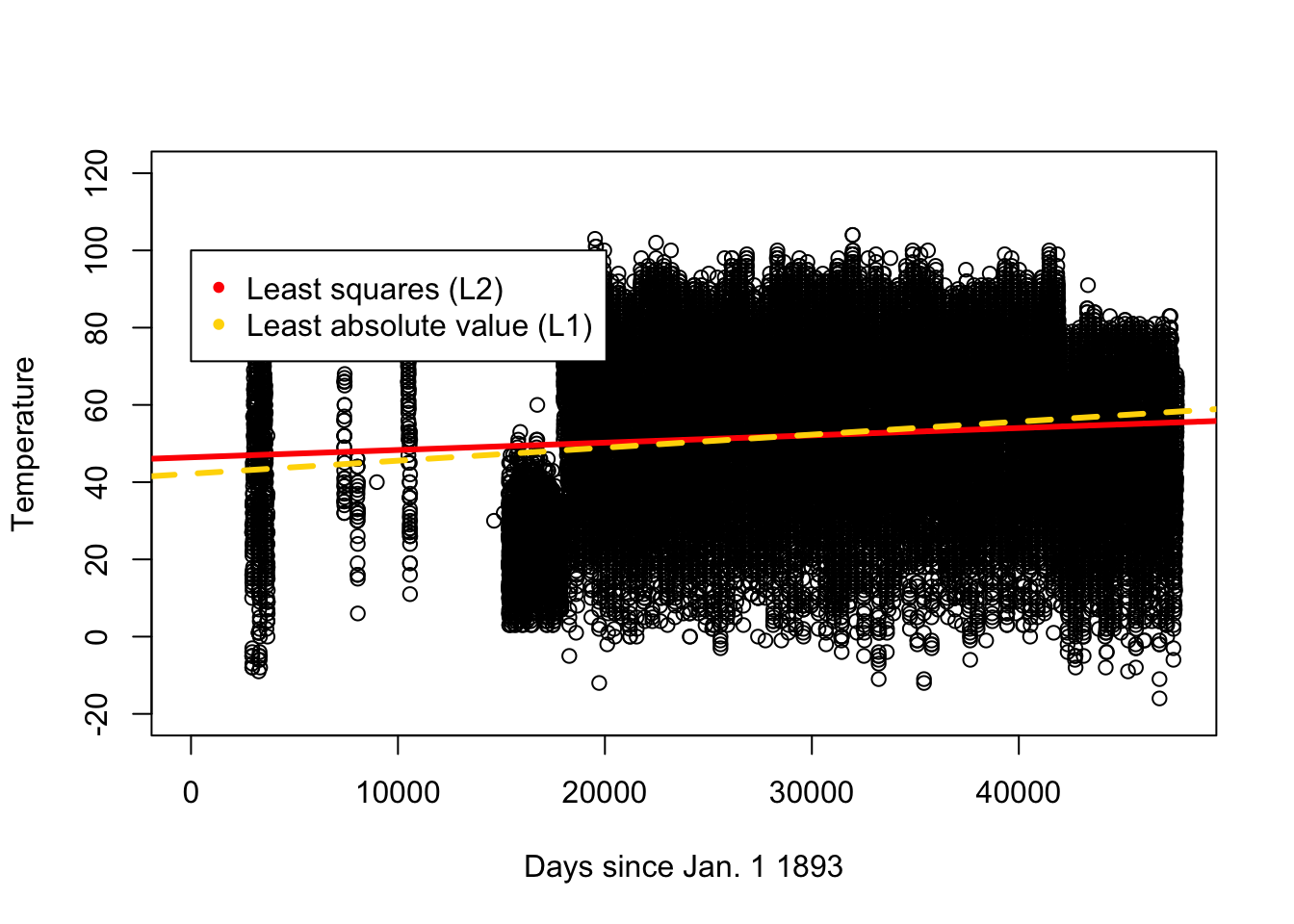
## NULL

plot(df.temp$days,df.temp$TOBS,xlab="Days since Jan. 1 1893",ylab="Temperature",ylim=c(-20,120))
abline(a=46.42983,b=0.0001902842,col="red",lwd=3)
abline(a=42.18326,b=0.0003373865,col="gold",lwd=3,lty=2)
legend(0,100,legend=c("Least squares (L2)","Least absolute value (L1)"), col=c("red","gold"),pch=20)

(d)

#Calculate number of days between 1/1/2050 and 1/1/1883.
ymd("2050-1-1") - min(df.temp$DATE)

## Time difference of 57343 days

# Expected temperature using Least squares (L2)
46.42983+0.0001902842*57343

## [1] 57.3413

# # Expected temperature using Least absolute value (L1)
42.18326+0.0003373865*57343

## [1] 61.53001

All linear models used in this assignment related to the temperature data used a loss function approach for estimation. The loss function approach enables the estimation of parameters (e.g., slopes and intercepts) that can be used to make predictions (e.g., the expected temperature in 2050). All of these estimates and prediction are single number (i.e., point estimates/predictions) and therefore do not use the concept of probabilistic thinking. We would need to make additional assumptions (e.g., error term in normally distributed) to obtain uncertainty quantification (e.g., confidence intervals and predictions intervals) that would enable the use of probabilistic thinking.