37 Day 36 (July 26)
37.2 Regression trees
- Example: Change point analysis
- Motivation: Annual mean temperature in Ann Arbor Michigan
library(faraway)
plot(aatemp$year,aatemp$temp,xlab="Year",ylab="Annual mean temperature",pch=20,col=rgb(0.5,0.5,0.5,0.7))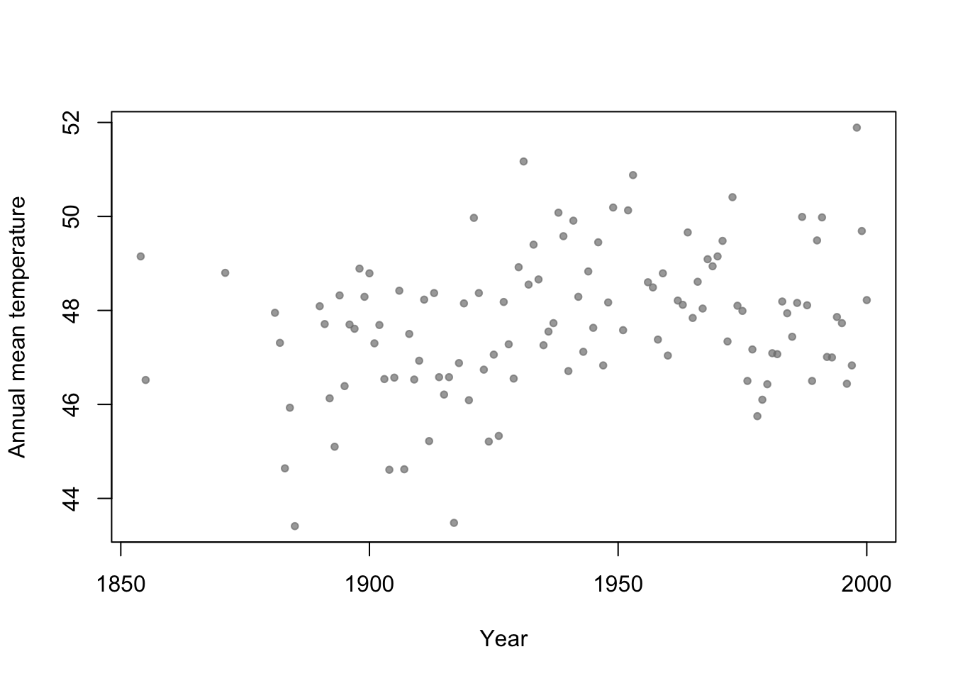
- Basis function \[f_1(x)=\begin{cases} 1 & \text{if}\;x<c\\ 0 & \text{otherwise} \end{cases}\] and \[f_2(x)=\begin{cases} 1 & \text{if}\;x\geq c\\ 0 & \text{otherwise} \end{cases}\]
- In R
# Change point basis function
f1 <- function(x,c){ifelse(x<c,1,0)}
f2 <- function(x,c){ifelse(x>=c,1,0)}

# Fit linear model
m1 <- lm(temp ~ -1 + f1(year,1930) + f2(year,1930),data=aatemp)
summary(m1)
## ## Call: ## lm(formula = temp ~ -1 + f1(year, 1930) + f2(year, 1930), data = aatemp) ## ## Residuals: ## Min 1Q Median 3Q Max ## -3.5467 -0.8962 -0.1157 1.1388 3.5843 ## ## Coefficients: ## Estimate Std. Error t value Pr(>|t|) ## f1(year, 1930) 46.9567 0.1990 236.0 <2e-16 *** ## f2(year, 1930) 48.3057 0.1684 286.8 <2e-16 *** ## --- ## Signif. codes: 0 '***' 0.001 '**' 0.01 '*' 0.05 '.' 0.1 ' ' 1 ## ## Residual standard error: 1.378 on 113 degrees of freedom ## Multiple R-squared: 0.9992, Adjusted R-squared: 0.9992 ## F-statistic: 6.899e+04 on 2 and 113 DF, p-value: < 2.2e-16# Plot predictions plot(aatemp$year,aatemp$temp,xlab="Year",ylab="Annual mean temperature",pch=20,col=rgb(0.5,0.5,0.5,0.7)) points(aatemp$year,predict(m1),type="l")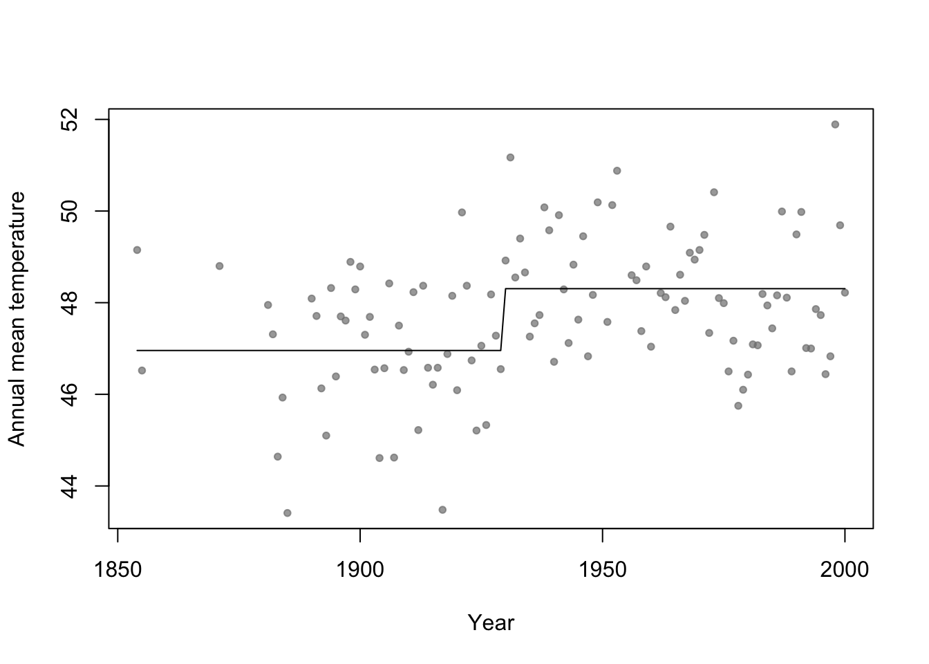
- Connection to regression trees
- For a single predictor, a regression tree can be though of as a linear model that uses the “change point” basis function, but tries to estimate the location (or time) and number of change points.
- Example in R
library(rpart)

# Fit regression tree model
m2 <- rpart(temp ~ year,data=aatemp)

# Plot predictions
E.y <- predict(m2,data.frame(year=seq(1850,2023,by=1)))
plot(aatemp$year,aatemp$temp,xlab="Year",ylab="Annual mean temperature",pch=20,col=rgb(0.5,0.5,0.5,0.7),xlim=c(1850,2023))
points(1850:2023,E.y,type="l")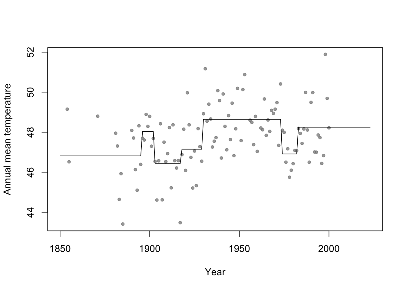
37.3 Random forest
Breiman 2001 link
Example
n.boot <- 1000 # Number of bootstrap samples
x.new=seq(1850,2023,by=1) # New values of x that I want predicitons at
E.y <- matrix(,length(x.new),n.boot) # Matrix to save predictions
x <- aatemp$year
y <- aatemp$temp

for(i in 1:n.boot){

  # Resample data
  df.temp <- data.frame(y=y,x=x)[sample(1:length(y),replace=TRUE,size=51),]

  # Fit tree
  m1 <- rpart(y~x,data=df.temp)

  # Get and save predictions
  E.y[,i] <- predict(m1,data.frame(x=x.new))
}

plot(aatemp$year,aatemp$temp,xlab="Year",ylab="Annual mean temperature",pch=20,col=rgb(0.5,0.5,0.5,0.7),xlim=c(1850,2023))


# Aggregate predictions
E.E.y <- rowMeans(E.y)
points(1850:2023,E.E.y,type="l")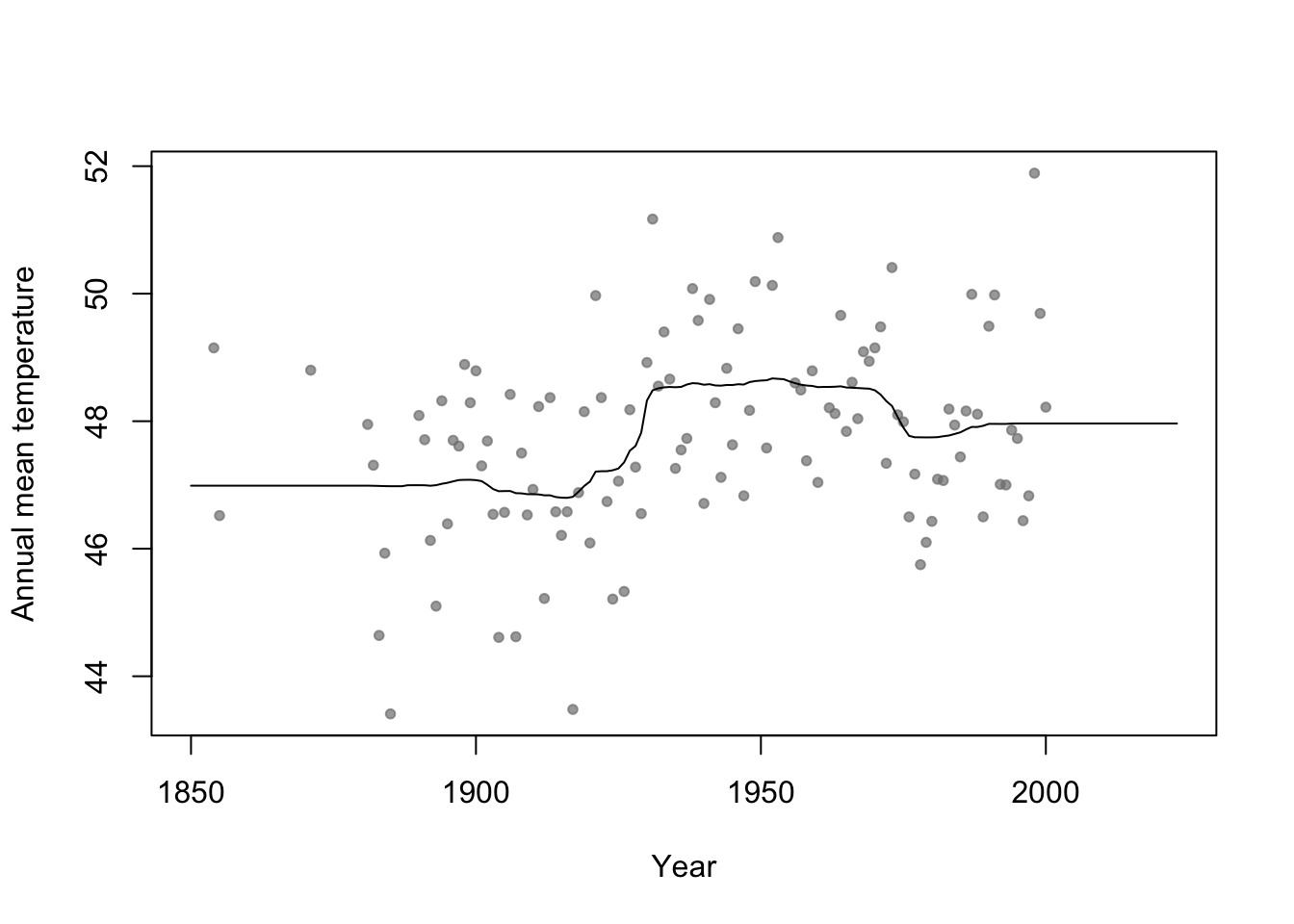
Summary
- Bootstrap aggregating (or bagging) can be used with any statistical model
- Usually increases predictive accuracy but reduces ability to understand (and write-out) the model(s) and make inference
37.4 Generalized additive model
Write out on white board
Difference between interpretable vs. non-interpretable model/machine learning approaches
My personal use of gams
- The functions lm() and glm() and packages lme4, nlme, etc
- Why I use the mgcv package
- Wood (2017)
- The functions lm() and glm() and packages lme4, nlme, etc
Example
library(faraway)
library(mgcv)

m1 <- gam(temp ~ s(year,bs="tp"),family=Gamma(link="log"),data=aatemp)

# Plot predictions
E.y <- predict(m1,data.frame(year=seq(1850,2023,by=1)),type="response")
ui <- E.y + 1.96*predict(m1,data.frame(year=seq(1850,2023,by=1)),type="response",se=TRUE)$se.fit
li <- E.y - 1.96*predict(m1,data.frame(year=seq(1850,2023,by=1)),type="response",se=TRUE)$se.fit
plot(aatemp$year,aatemp$temp,xlab="Year",ylab="Annual mean temperature",pch=20,col=rgb(0.5,0.5,0.5,0.7),xlim=c(1850,2023))
points(1850:2023,E.y,type="l",lwd=3)
points(1850:2023,ui,type="l",lwd=2,lty=2)
points(1850:2023,li,type="l",lwd=2,lty=2)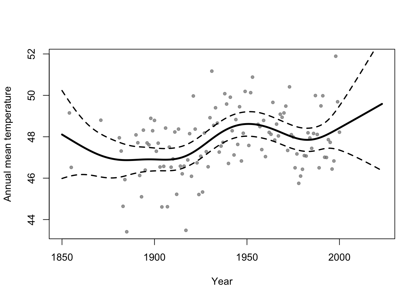
37.5 Shrinkage methods
Ridge regression (Hoerl and Kennard 1970)
- See pgs. 174-177 of Chapter 11 in (Faraway 2014)
- Minimize the loss function \[\underset{\boldsymbol{\beta}}{\operatorname{argmin}} (\mathbf{y}-\mathbf{X}\boldsymbol{\beta})^{'}(\mathbf{y}-\mathbf{X}\boldsymbol{\beta})+\lambda\sum_{j=1}^{p}\beta_{j}^{2}\]
- Properties of ridge regression
- Connection to the linear model with random effects
- \(\hat{\boldsymbol{\beta}}=\left(\mathbf{X}^{'}\mathbf{X}+\lambda\mathbf{I}\right)^{-1}\mathbf{X}^{'}\mathbf{y}\)
- \(\text{rank}(\mathbf{X}^{'}\mathbf{X}+\lambda\mathbf{I})\)
- \(\hat{\boldsymbol{\beta}}\) when \(\lambda=0\)
- \(\hat{\boldsymbol{\beta}}\) when \(\lambda=\infty\)
- Recall \[\begin{equation} \begin{split} \hat{\text{E}(\mathbf{y})} & = \mathbf{X}\hat{\boldsymbol{\beta}} \\ & = \mathbf{X}\left(\mathbf{X}^{\prime}\mathbf{X}+\lambda\mathbf{I}\right)^{-1}\mathbf{X}^{\prime}\mathbf{y}\\ & = \mathbf{H}\mathbf{y}\\ \end{split} \end{equation}\]
- Effective number of coefficients \(=\text{trace}(\mathbf{H})\)
- If \(\lambda=0\), then \(\text{trace}(\mathbf{H}) = \text{?}\)
- If \(\lambda=\infty\), then \(\text{trace}(\mathbf{H}) = \text{?}\)
- Estimation requires selecting a value for \(\lambda\)
- Example: Variable selection and dealing with collinearity
- Linear model with \(\lambda=0\)
library(httr)
library(readxl)

url <- "https://doi.org/10.1371/journal.pone.0148743.s005"
GET(url, write_disk(path <- tempfile(fileext = ".xls")))
df1 <- read_excel(path = path, sheet = "Data", col_names = TRUE, col_types = "numeric") df1 <- df1[complete.cases(df1),]## ## Call: ## lm(formula = CDEP ~ NCAT + WPOP + WKIL, data = df1) ## ## Residuals: ## Min 1Q Median 3Q Max ## -18.483 -9.151 -1.477 3.985 78.775 ## ## Coefficients: ## Estimate Std. Error t value Pr(>|t|) ## (Intercept) 14.5176798 6.6712280 2.176 0.0339 * ## NCAT -0.0014333 0.0008412 -1.704 0.0941 . ## WPOP 0.0108041 0.0159751 0.676 0.5017 ## WKIL 0.6864227 0.0985674 6.964 4.71e-09 *** ## --- ## Signif. codes: 0 '***' 0.001 '**' 0.01 '*' 0.05 '.' 0.1 ' ' 1 ## ## Residual standard error: 14.95 on 54 degrees of freedom ## Multiple R-squared: 0.7784, Adjusted R-squared: 0.7661 ## F-statistic: 63.23 on 3 and 54 DF, p-value: < 2.2e-16## NCAT WPOP WKIL ## NCAT 1.00000000 -0.3547717 -0.05005347 ## WPOP -0.35477170 1.0000000 0.79070496 ## WKIL -0.05005347 0.7907050 1.00000000- Linear model with \(\lambda=10\)
## ## Call: ## lm(formula = y ~ X) ## ## Residuals: ## Min 1Q Median 3Q Max ## -18.483 -9.151 -1.477 3.985 78.775 ## ## Coefficients: ## Estimate Std. Error t value Pr(>|t|) ## (Intercept) 28.776 1.964 14.655 < 2e-16 *** ## XNCAT -3.944 2.314 -1.704 0.0941 . ## XWPOP 2.554 3.776 0.676 0.5017 ## XWKIL 24.615 3.535 6.964 4.71e-09 *** ## --- ## Signif. codes: 0 '***' 0.001 '**' 0.01 '*' 0.05 '.' 0.1 ' ' 1 ## ## Residual standard error: 14.95 on 54 degrees of freedom ## Multiple R-squared: 0.7784, Adjusted R-squared: 0.7661 ## F-statistic: 63.23 on 3 and 54 DF, p-value: < 2.2e-16## XNCAT XWPOP XWKIL ## 28.775862 -2.243853 7.196794 17.936405- Ridge regression using glmnet() and multiple values of \(\lambda\)
library(glmnet)
lambda <- seq(0,400,by=0.1)
m4 <- glmnet(X,y,family=c("gaussian"),alpha=0,standardize=FALSE,lambda=lambda)
plot(m4, xvar = "lambda", label = TRUE)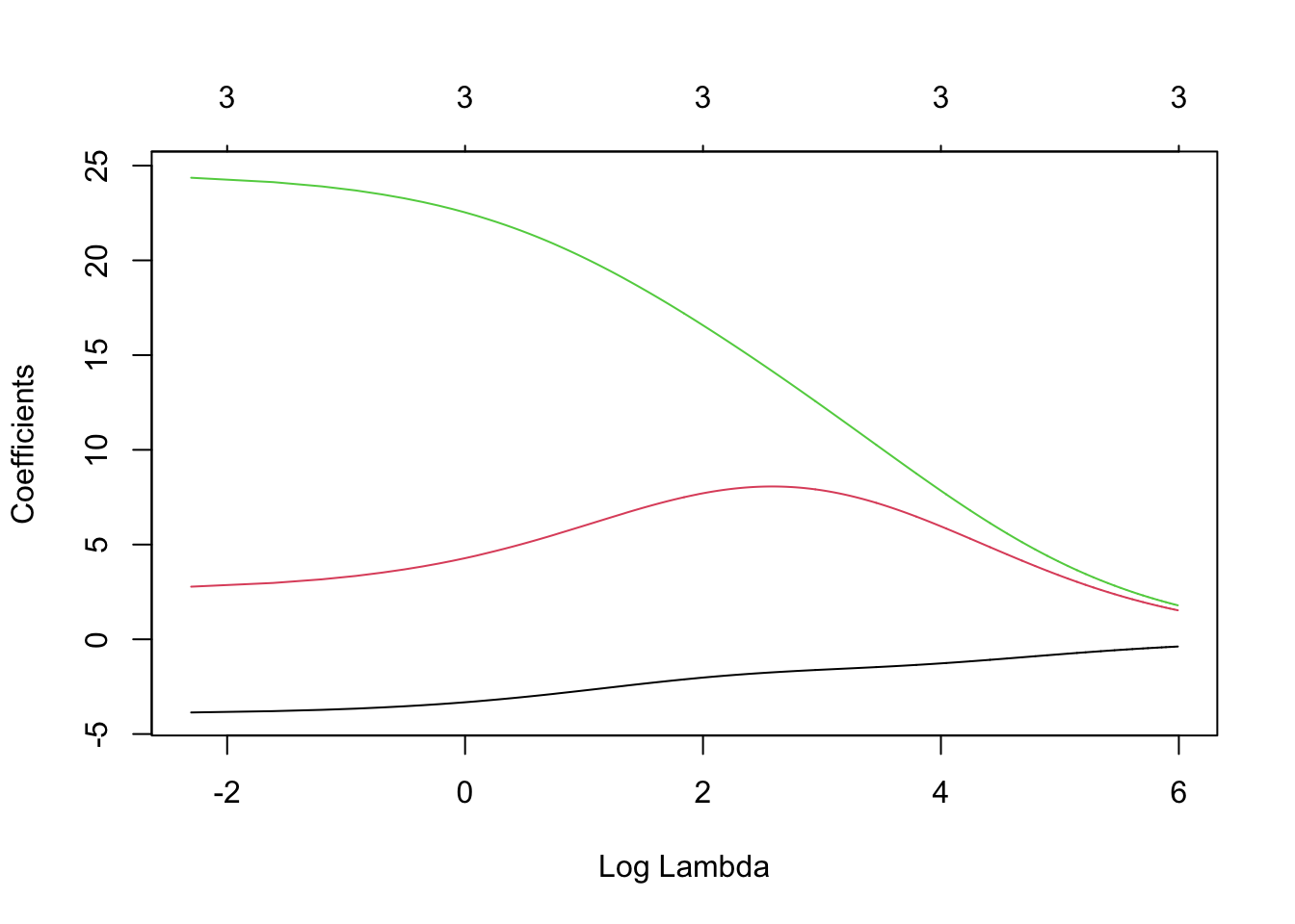
- Ridge regression using 10 fold cross-validation
m5 <- cv.glmnet(X,y,family=c("gaussian"),alpha=0,standardize=FALSE,lambda=lambda,nfolds = 10)
plot(m5)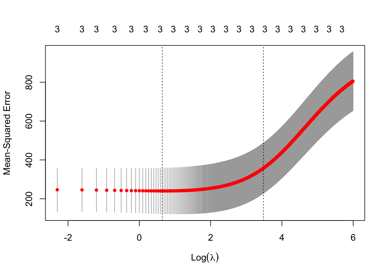
## [1] 1.9## 4 x 1 sparse Matrix of class "dgCMatrix" ## s0 ## (Intercept) 28.775862 ## NCAT -2.950257 ## WPOP 5.314891 ## WKIL 21.147750LASSO (Tibshirani 1996)
- Minimize the loss function \[\underset{\boldsymbol{\beta}}{\operatorname{argmin}} (\mathbf{y}-\mathbf{X}\boldsymbol{\beta})^{'}(\mathbf{y}-\mathbf{X}\boldsymbol{\beta})+\lambda\sum_{j=1}^{p}|\beta_{j}|\]
- Properties of LASSO
- Connection to the linear model with random effects
- No closed-form solution for \(\hat{\boldsymbol{\beta}}\)
- Shrinks and selects (Least Absolute Shrinkage and Selection Operator)
- Good to use when collinearity is not a huge problem and when some of the \(\boldsymbol{\beta}\) are thought to be zero.
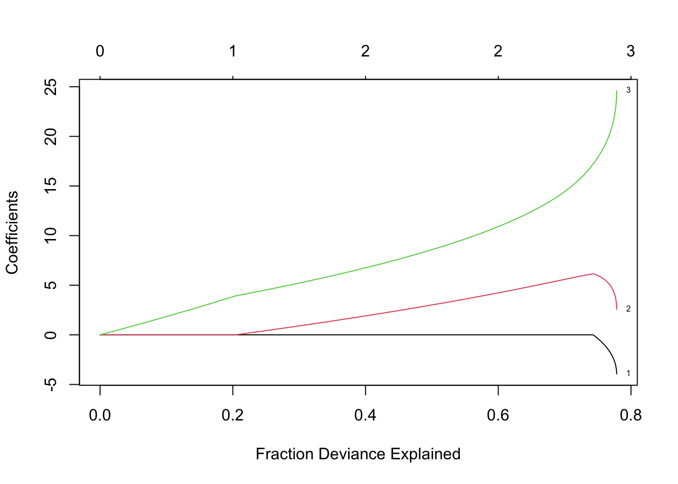
- Example: LASSO using glmnet() and multiple values of \(\lambda\)
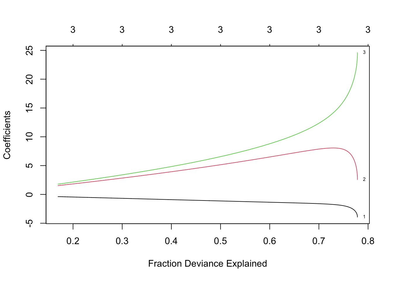
X <- scale(df1[,c(7,5,4)])
y <- df1$CDEP

library(glmnet)
lambda <- seq(0,400,by=0.1)
m7 <- glmnet(X,y,family=c("gaussian"),alpha=1,standardize=FALSE,lambda=lambda)
plot(m7, xvar = "lambda", label = TRUE)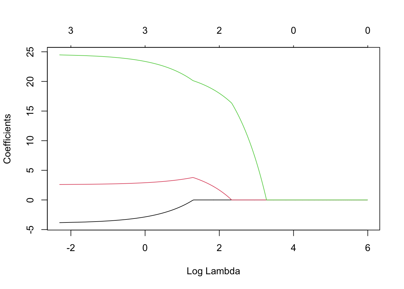
 - LASSO using 10 fold cross-validation
m8 <- cv.glmnet(X,y,family=c("gaussian"),alpha=1,standardize=FALSE,lambda=lambda,nfolds = 10)
plot(m8)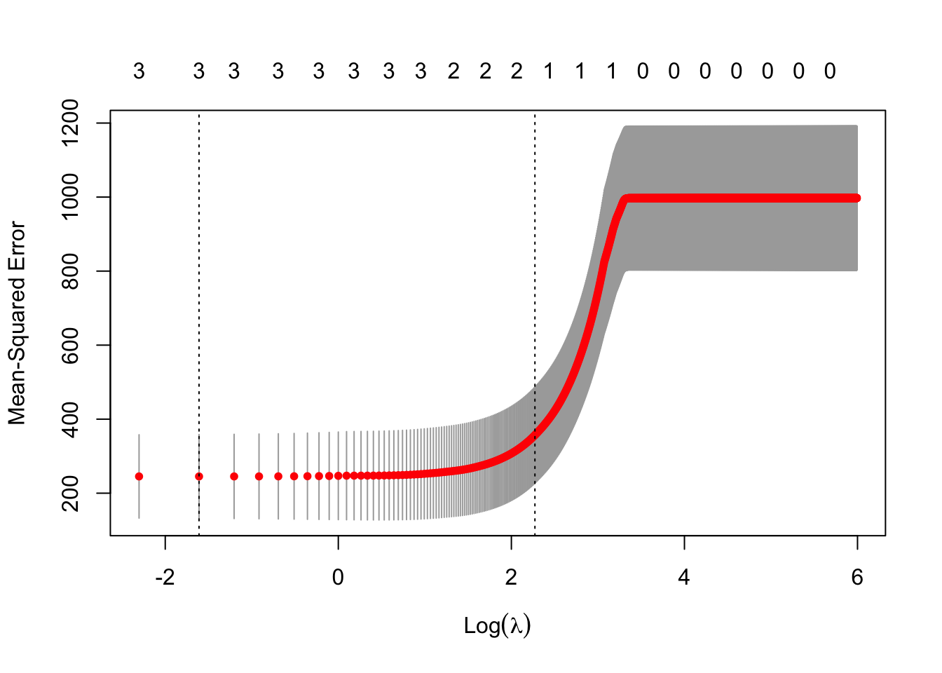
## [1] 0.2## 4 x 1 sparse Matrix of class "dgCMatrix" ## s0 ## (Intercept) 28.775862 ## NCAT -3.722689 ## WPOP 2.634395 ## WKIL 24.358870## 4 x 1 sparse Matrix of class "dgCMatrix" ## s0 ## (Intercept) 28.7758621 ## NCAT . ## WPOP 0.3655531 ## WKIL 16.6725216Elastic net (Zou and Hastie 2005)
- Mix of ridge and lasso penalty
- Example: Elastic net using glmnet() and multiple values of \(\lambda\)
lambda <- seq(0,400,by=0.1)
m11 <- glmnet(X,y,family=c("gaussian"),alpha=0.5,standardize=FALSE,lambda=lambda)
plot(m11, xvar = "lambda", label = TRUE)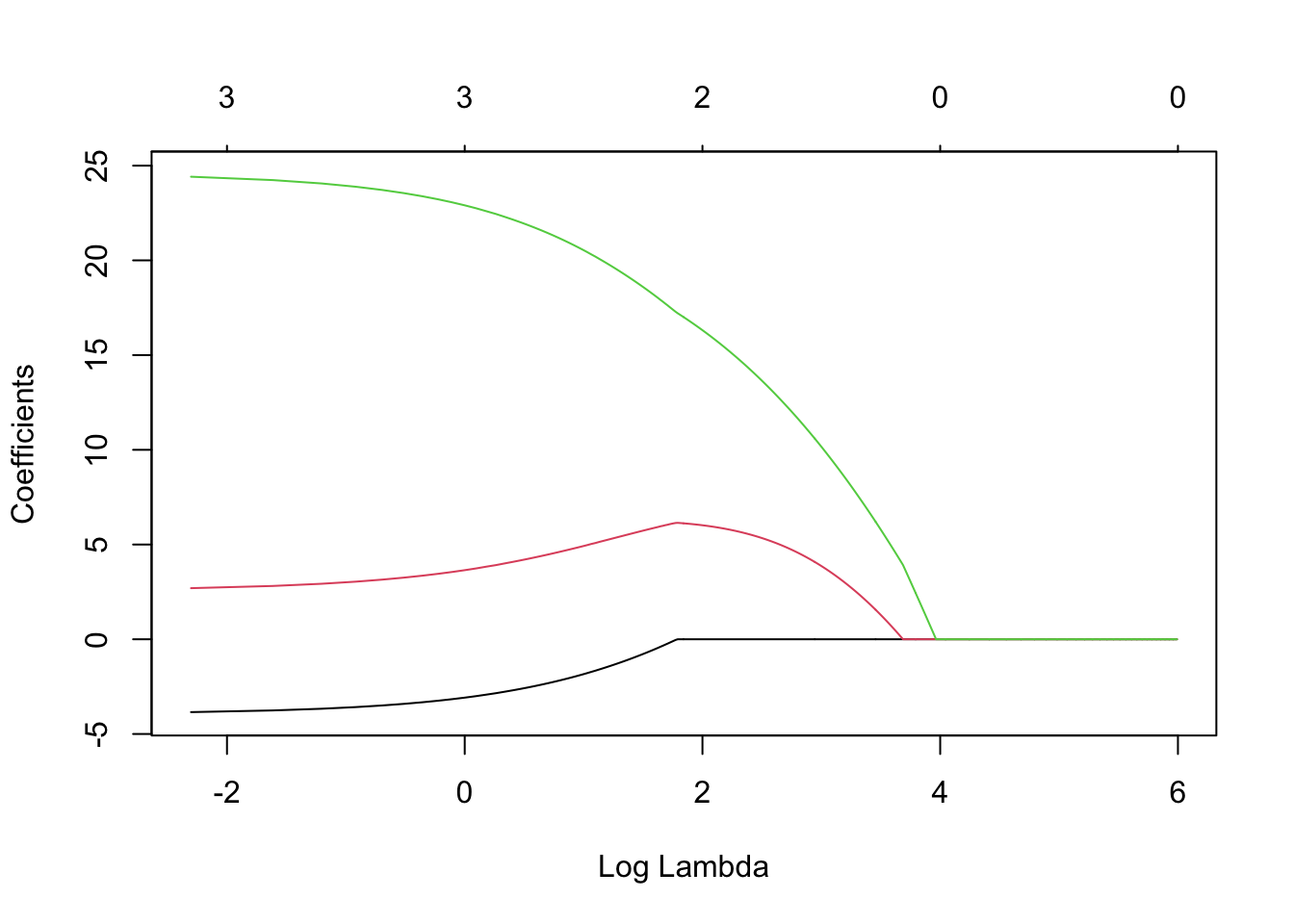
 - Elastic net using 10 fold cross-validation
m12 <- cv.glmnet(X,y,family=c("gaussian"),alpha=1,standardize=FALSE,lambda=lambda,nfolds = 10)
plot(m11)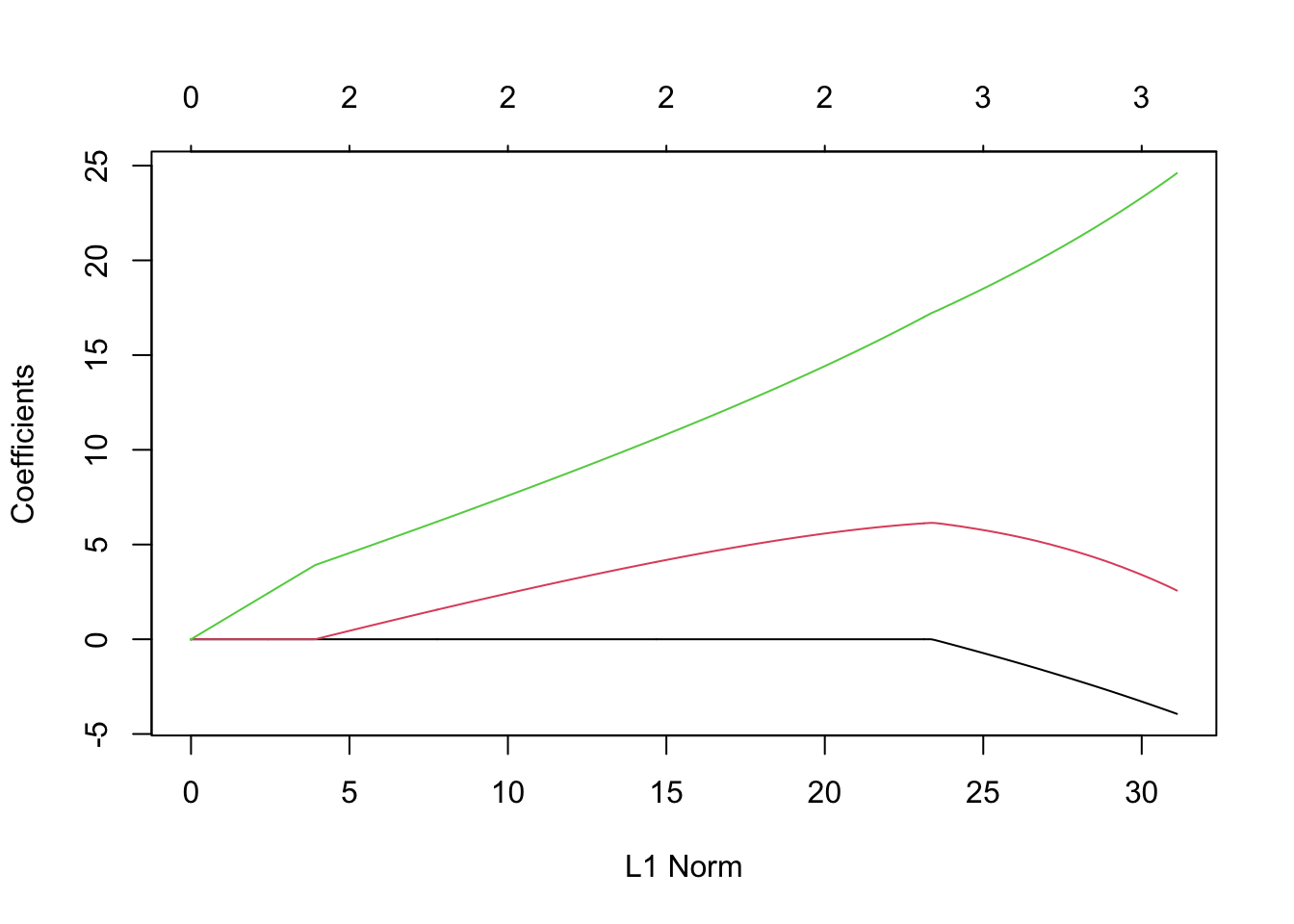
## [1] 1.4## 4 x 1 sparse Matrix of class "dgCMatrix" ## s0 ## (Intercept) 28.775862 ## NCAT -2.431400 ## WPOP 3.039959 ## WKIL 22.881770Summary
- Non-Bayesian inference (e.g., confidence intervals) is an open question
- Methods that shrink coefficients can be used to introduce bias which reduces variance
- Methods that do continuous shrinkage are preferend to binary shrinkage (e.g., variable selection with AIC).
- Shrinking coefficients is one way to deal with collinearity.
- Most continuous shrinkage methods are some gernalization of ridge or LASSO penalty.
- Good references
Literature cited
Faraway, J. J. 2014. Linear Models with r. CRC Press.
Hoerl, Arthur E, and Robert W Kennard. 1970. “Ridge Regression: Biased Estimation for Nonorthogonal Problems.” Technometrics 12 (1): 55–67.
Tibshirani, Robert. 1996. “Regression Shrinkage and Selection via the Lasso.” Journal of the Royal Statistical Society. Series B (Methodological), 267–88.
Zou, Hui, and Trevor Hastie. 2005. “Regularization and Variable Selection via the Elastic Net.” Journal of the Royal Statistical Society: Series B (Statistical Methodology) 67 (2): 301–20.