21 Day 21 (July 2)

21.1 Announcements

• Read Chs. 14, 15 and 16 in linear models with R

• Next read Ch. 6 (Model diagnostics) in Linear models with R

• Guide for assignment 3 is posted.

21.2 ANOVA/F-test

• F-test (pgs. 33 - 39 in Faraway (2014))

  • The t-test is useful for testing simple hypotheses
  • F-test is useful for testing more complicated hypotheses
  • Example: comparing more than two means

  library(faraway)
  boxplot(weight ~ group, data=PlantGrowth,col="grey",ylim=c(0,7))

  

  aggregate(weight ~ group, FUN=mean,data=PlantGrowth)

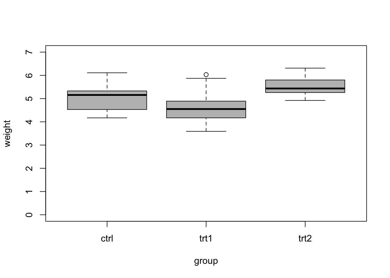
  ##   group weight
  ## 1  ctrl  5.032
  ## 2  trt1  4.661
  ## 3  trt2  5.526

  To determine if treatment 1 and 2 had an effects, we might propose the following null hypothesis \[\text{H}_{0}:\beta_1 = \beta_2 = 0\] and alternative hypothesis \[\text{H}_{\text{a}}:\beta_1 \neq 0 \;\text{or}\; \beta_2 \neq 0.\] To test the null hypothesis, we calculate the probability that we observe values of \(\hat{\beta_1}\) and \(\hat{\beta_2}\) as or more extreme than the null hypothesis. To calculate this probability, note that \[\frac{(TSS - RSS)/(p-1)}{RSS/(n-1)} \sim\text{F}(p-1,n-p).\] The probability that we observe a value of \(\hat{\beta_1}\) and \(\hat{\beta_2}\) as or more extreme than the null hypothesis can be written as \[\text{P}\bigg(\frac{(TSS - RSS)/(p-1)}{RSS/(n-1)} <F\bigg),\] where \(TSS = (\mathbf{y} - \bar{\mathbf{y}})^{\prime}(\mathbf{y} - \bar{\mathbf{y}})\) and \(RSS = (\mathbf{y} - \mathbf{X}\hat{\boldsymbol{\beta}})^{\prime}(\mathbf{y} - \mathbf{X}\hat{\boldsymbol{\beta}})\). The probability can be calculated as the area under the curve of a F-distribution. The code below shows how to do these calculations in R

  m1 <- lm(weight ~ group,data = PlantGrowth)
  summary(m1)

  ## 
  ## Call:
  ## lm(formula = weight ~ group, data = PlantGrowth)
  ## 
  ## Residuals:
  ##     Min      1Q  Median      3Q     Max 
  ## -1.0710 -0.4180 -0.0060  0.2627  1.3690 
  ## 
  ## Coefficients:
  ##             Estimate Std. Error t value Pr(>|t|)    
  ## (Intercept)   5.0320     0.1971  25.527   <2e-16 ***
  ## grouptrt1    -0.3710     0.2788  -1.331   0.1944    
  ## grouptrt2     0.4940     0.2788   1.772   0.0877 .  
  ## ---
  ## Signif. codes:  0 '***' 0.001 '**' 0.01 '*' 0.05 '.' 0.1 ' ' 1
  ## 
  ## Residual standard error: 0.6234 on 27 degrees of freedom
  ## Multiple R-squared:  0.2641, Adjusted R-squared:  0.2096 
  ## F-statistic: 4.846 on 2 and 27 DF,  p-value: 0.01591

  anova(m1)

  ## Analysis of Variance Table
  ## 
  ## Response: weight
  ##           Df  Sum Sq Mean Sq F value  Pr(>F)  
  ## group      2  3.7663  1.8832  4.8461 0.01591 *
  ## Residuals 27 10.4921  0.3886                  
  ## ---
  ## Signif. codes:  0 '***' 0.001 '**' 0.01 '*' 0.05 '.' 0.1 ' ' 1

  # "By hand"
  beta.hat <- coef(m1)
  X <- model.matrix(m1)
  y <- PlantGrowth$weight
  y.bar <- mean(y)
  n <- 30
  p <- 3
  
  
  RSS <- t(y-X%*%beta.hat)%*%(y-X%*%beta.hat)
  RSS

  ##          [,1]
  ## [1,] 10.49209

  TSS <- t(y-y.bar)%*%(y-y.bar)
  TSS

  ##          [,1]
  ## [1,] 14.25843

  TSS-RSS

  ##         [,1]
  ## [1,] 3.76634

  F <- ((TSS - RSS)/(p-1))/(RSS/(n-p))
  F

  ##          [,1]
  ## [1,] 4.846088

  pf(F,p-1,n-p,lower.tail=FALSE)

  ##            [,1]
  ## [1,] 0.01590996

• Live example

  • Research publication
  • Data
  • R Script

21.3 Model checking

• Given a statistical model, estimation, prediction, and statistical inference is somewhat “automatic”
• If the statistical model is misspecified (i.e., wrong) in any way, the resulting statistical inference (including predictions and prediction uncertainty) rests on a house of cards.
• George Box quote: “All models are wrong but some are useful.”
  • Box (1976) “Since all models are wrong the scientist cannot obtain a correct one by excessive elaboration. On the contrary following William of Occam he should seek an economical description of natural phenomena. Just as the ability to devise simple but evocative models is the signature of the great scientist so overelaboration and overparameterization is often the mark of mediocrity.”
• We have assumed the linear model \(\mathbf{y}\sim\text{N}(\mathbf{X\boldsymbol{\beta}},\sigma^{2}\mathbf{I})\), which allowed us to:
  • Estimate \(\boldsymbol{\beta}\) and \(\sigma^2\)
  • Make statistical inference about \(\hat{\boldsymbol{\beta}}\)
  • Make predictions and obtain prediction intervals for future values of \(\mathbf{y}\)
• All statistical inference we obtained requires that the linear model \(\mathbf{y}\sim\text{N}(\mathbf{X\boldsymbol{\beta}},\sigma^{2}\mathbf{I})\) gave rise to the data.
  • Support
  • Linear
  • Constant variance
  • Independence
  • Outliers
• Model diagnostics (Ch 6 in Faraway (2014)) is a set of tools and procedures to see if the assumptions of our model are approximately correct.
  • Statistical tests (e.g., Shapiro-Wilk test for normality)
    • Specific
    • What if you reject the null?
  • Graphical
    • Broad
    • Subjective
    • Widely used
  • Predictive model checks
    • More common for Bayesian models (e.g., posterior predictive checks)
• We will explore numerous ways to check
  • Distributional assumptions
    • Normality
    • Constant variance
    • Correlation among errors
  • Detection of outliers
  • Deterministic model structure
    • Is \(\mathbf{X}\boldsymbol{\beta}\) a reasonable assumption?

References

Box, George EP. 1976. “Science and Statistics.” Journal of the American Statistical Association 71 (356): 791–99.

Faraway, J. J. 2014. Linear Models with r. CRC Press.