35 Day 34 (July 24)
35.1 Announcements
- Teval
- Final grades
- More about challenger example here
35.2 Transformations of the response
Big picture idea
- Select a function that transforms \(\mathbf{y}\) such that the assumptions of normality are approximately correct.
Two cultures
- This is with respect to \(\mathbf{y}\) and not the predictors. Transforming the predictors is not at all controversial.
- Trade offs
- Difficult to apply sometimes (e.g., \(\text{log(}\mathbf{y}+c)\) for count data)
- Difficult to interpret on the transformed scale
- If normality is an appropriate assumption, we can use the general linear model \(\textbf{y}\sim\text{N}(\mathbf{X}\boldsymbol{\beta},\mathbf{V})\)
Example
- Number of whooping cranes each year
url <- "https://www.dropbox.com/s/ihs3as87oaxvmhq/Butler%20et%20al.%20Table%201.csv?dl=1"
df1 <- read.csv(url)
plot(df1$Winter,df1$N,typ="b",xlab="Year",ylab="Population Size",ylim=c(0,300),lwd=1.5,pch="*")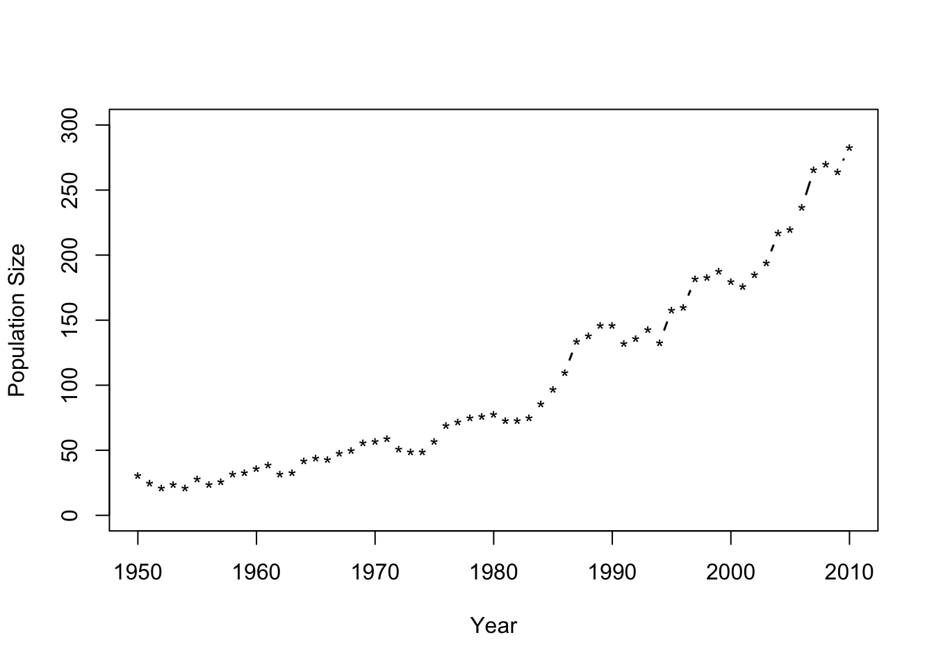
- Fit the model \(\mathbf{y}=\beta_{0}+\beta_{1}\mathbf{x}+\boldsymbol{\varepsilon}\) where \(\boldsymbol{\varepsilon}\sim\text{N}(\mathbf{0},\sigma^{2}\mathbf{I})\) and \(\mathbf{x}\) is the year.
m1 <- lm(N~Winter,data=df1)
plot(df1$Winter,df1$N,typ="b",xlab="Year",ylab="Population Size",ylim=c(0,300),lwd=1.5,pch="*")
abline(m1,col="gold")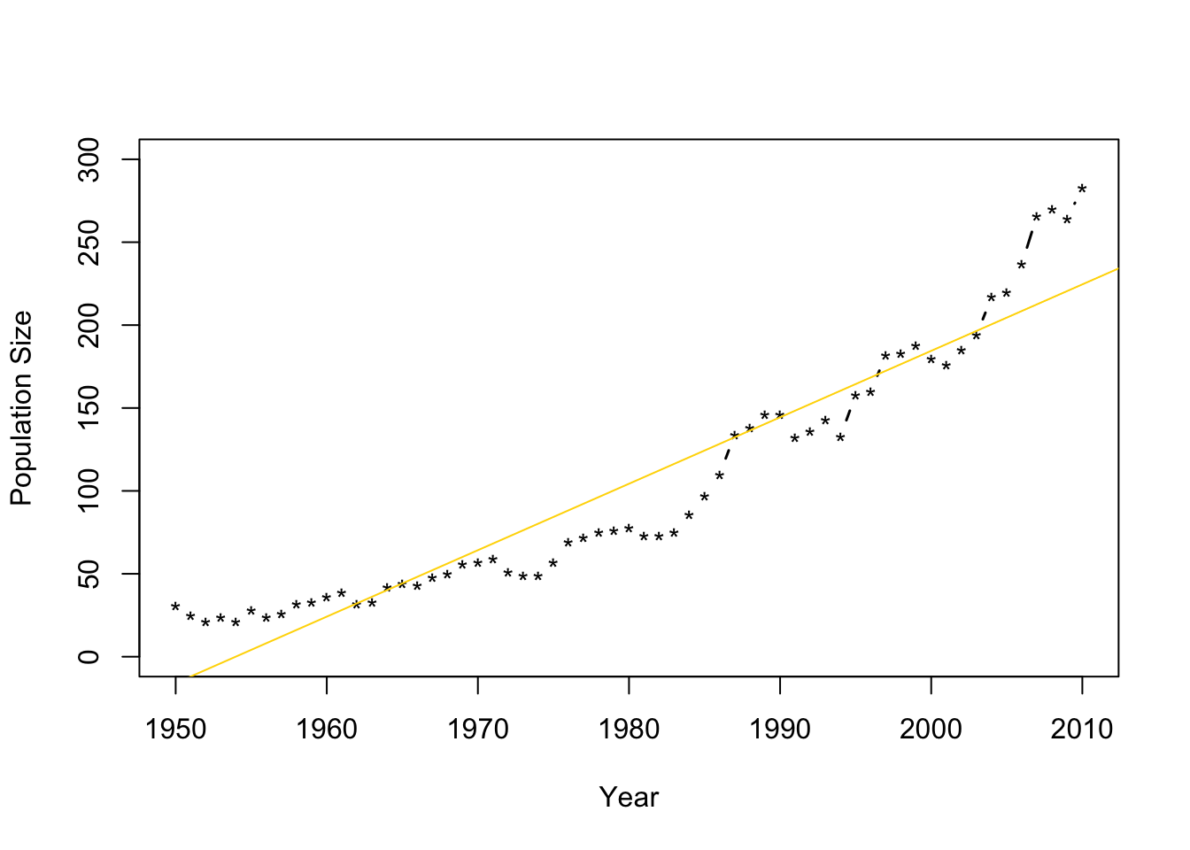
- Check model assumptions
e.hat <- residuals(m1)

#Check normality
hist(e.hat,col="grey",breaks=10,main="",xlab=expression(hat(epsilon)))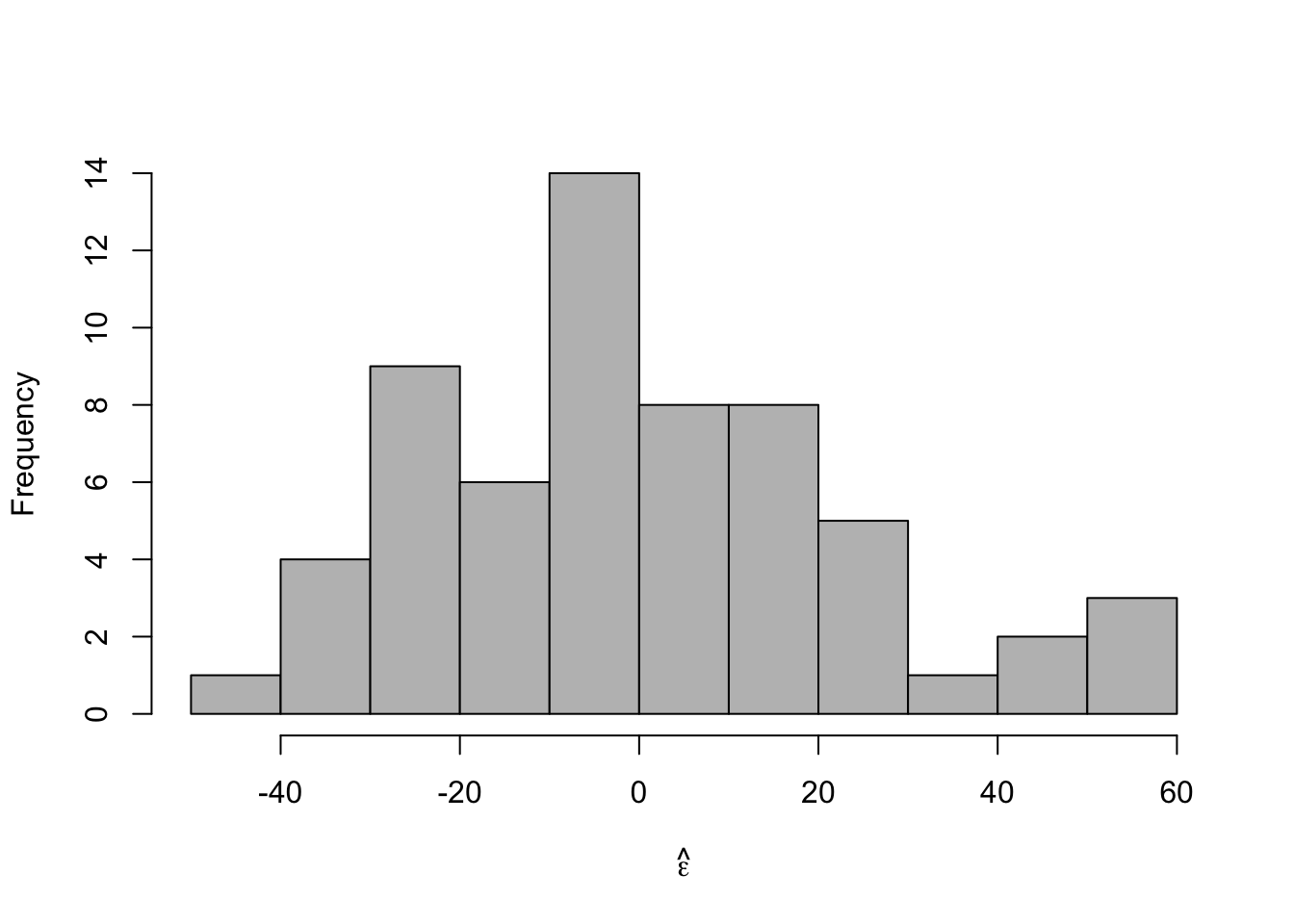
##
##  Shapiro-Wilk normality test
##
## data:  e.hat
## W = 0.96653, p-value = 0.09347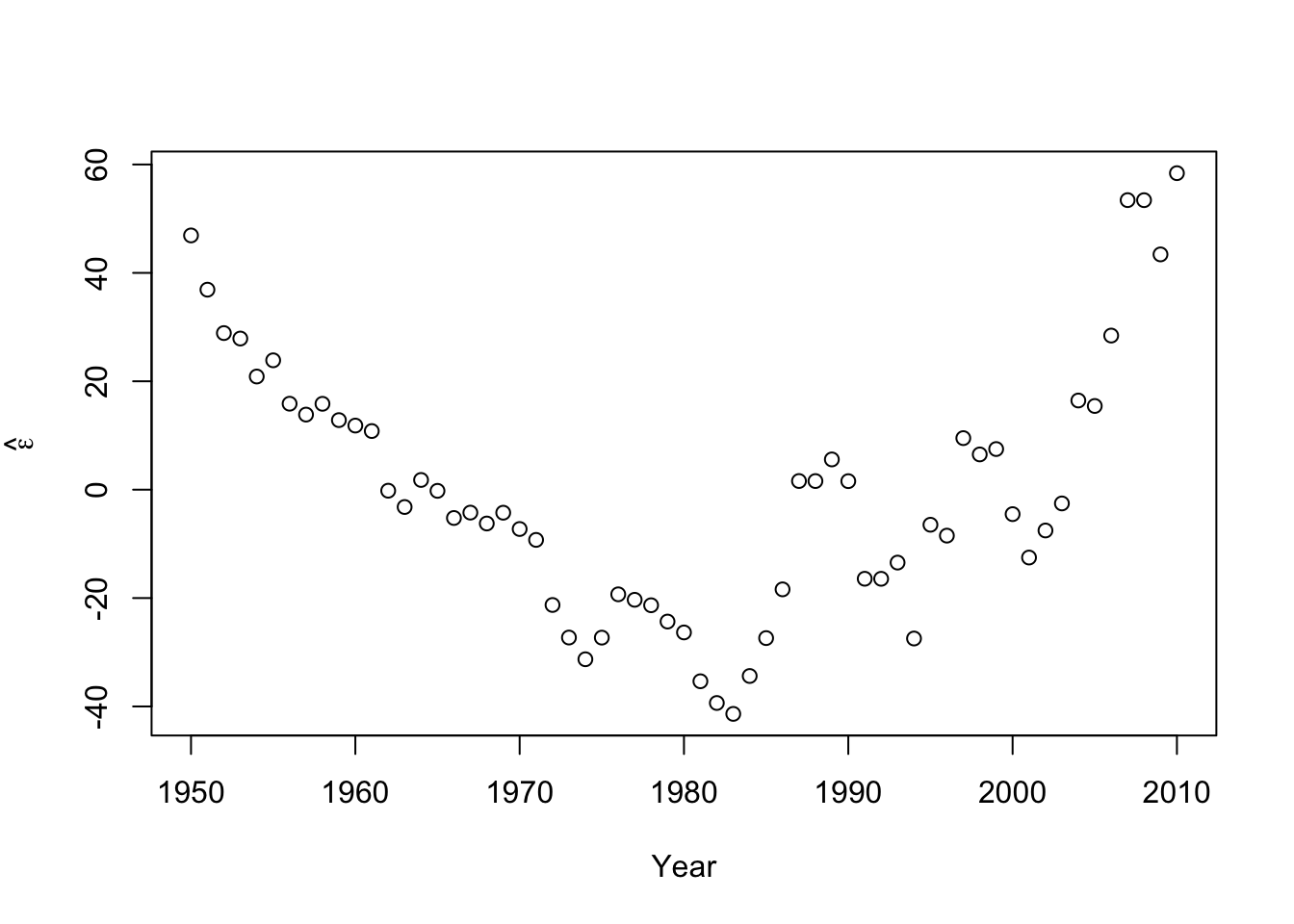
#Check for autocorrelation among residuals
plot(e.hat[1:60],e.hat[2:61],xlab=expression(hat(epsilon)[t]),ylab=expression(hat(epsilon)[t+1]))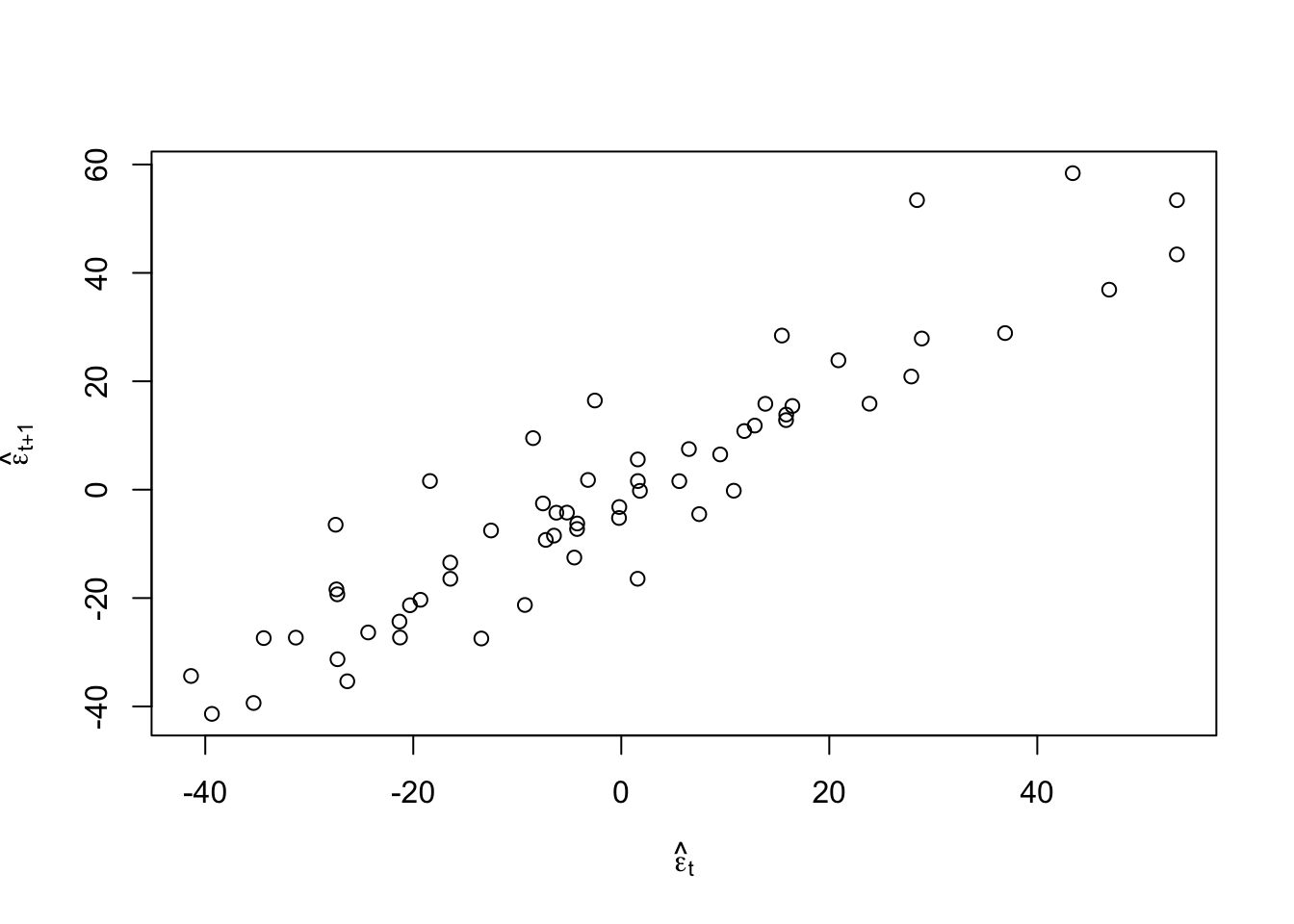
## [1] 0.9273559## ## Durbin-Watson test ## ## data: m1 ## DW = 0.13355, p-value < 2.2e-16 ## alternative hypothesis: true autocorrelation is greater than 0- Log transformation (i.e., \(\text{log}(\mathbf{y})\)).
- \(\text{log}(\mathbf{y})=\beta_{0}+\beta_{1}\mathbf{x}+\boldsymbol{\varepsilon}\) where \(\boldsymbol{\varepsilon}\sim\text{N}(\mathbf{0},\sigma^{2}\mathbf{I})\) and \(\mathbf{x}\) is the year.
- What model is implied by this transformation?
- If \(z\sim\text{N}(\mu,\sigma^{2})\), then \(\text{E}(e^{z})=e^{\mu+\frac{\sigma^{2}}{2}}\) and \(\text{Var}(e^{z})=(e^{\sigma^{2}}-1)e^{2\mu+\sigma^{2}}\)
- Fit the model
m2 <- lm(log(N)~Winter,data=df1) plot(df1$Winter,df1$N,typ="b",xlab="Year",ylab="Population Size",ylim=c(0,300),lwd=1.5,pch="*") abline(m1,col="gold") ev.y.hat <- exp(predict(m2)) # Possible because of invariance property of MLEs points(df1$Winter,ev.y.hat,typ="l",col="deepskyblue")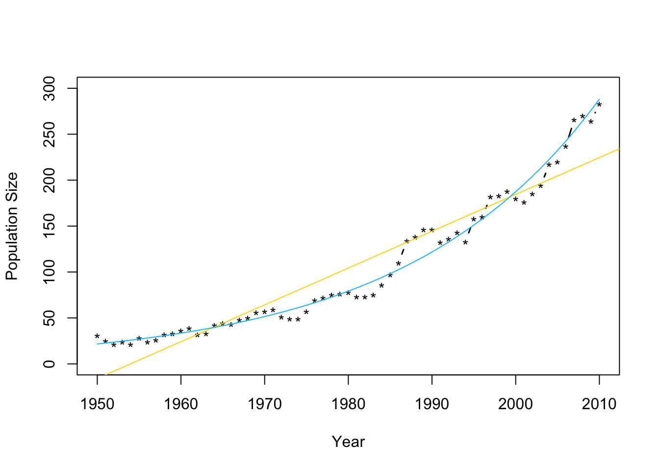 - Check model assumptions
e.hat <- residuals(m2)

#Check normality
hist(e.hat,col="grey",breaks=10,main="",xlab=expression(hat(epsilon)))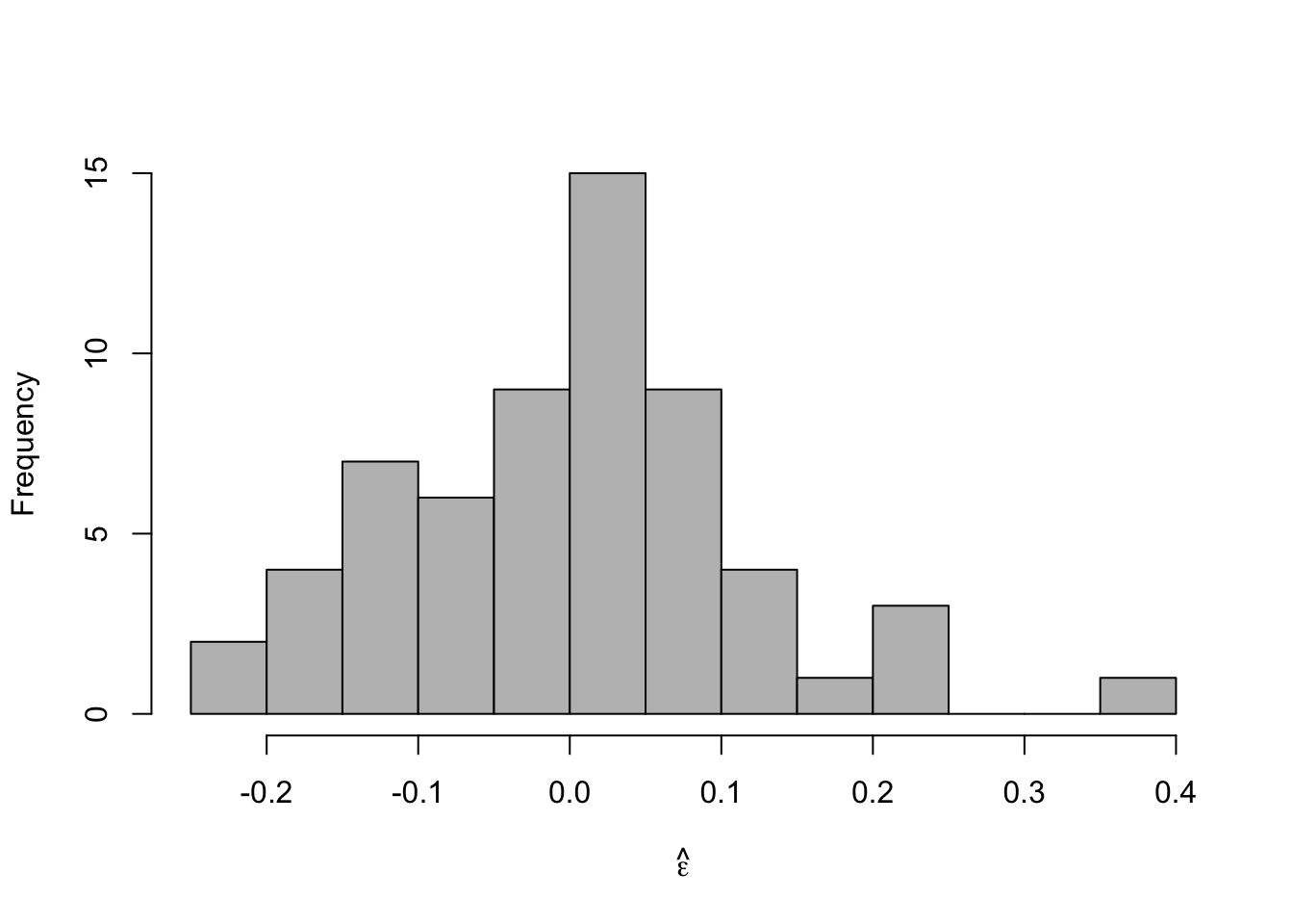
## ## Shapiro-Wilk normality test ## ## data: e.hat ## W = 0.97059, p-value = 0.1489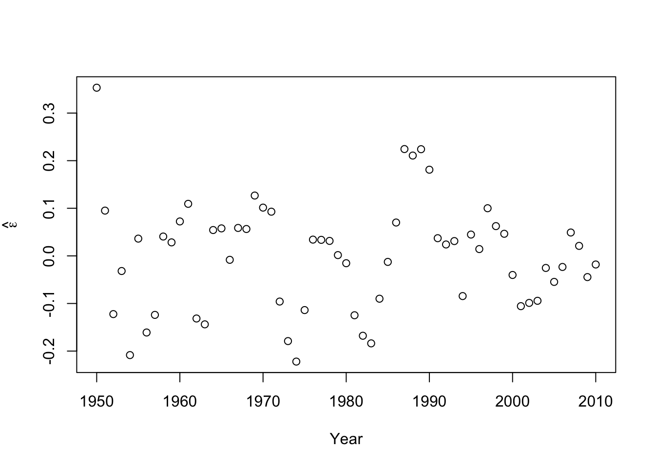 - Confidence intervals and prediction intervals
plot(df1$Winter,df1$N,typ="b",xlab="Year",ylab="Population Size",ylim=c(0,300),lwd=1.5,pch="*")
ev.y.hat <- exp(predict(m2)) # Possible because of invariance property of MLEs
points(df1$Winter,ev.y.hat,typ="l",col="deepskyblue")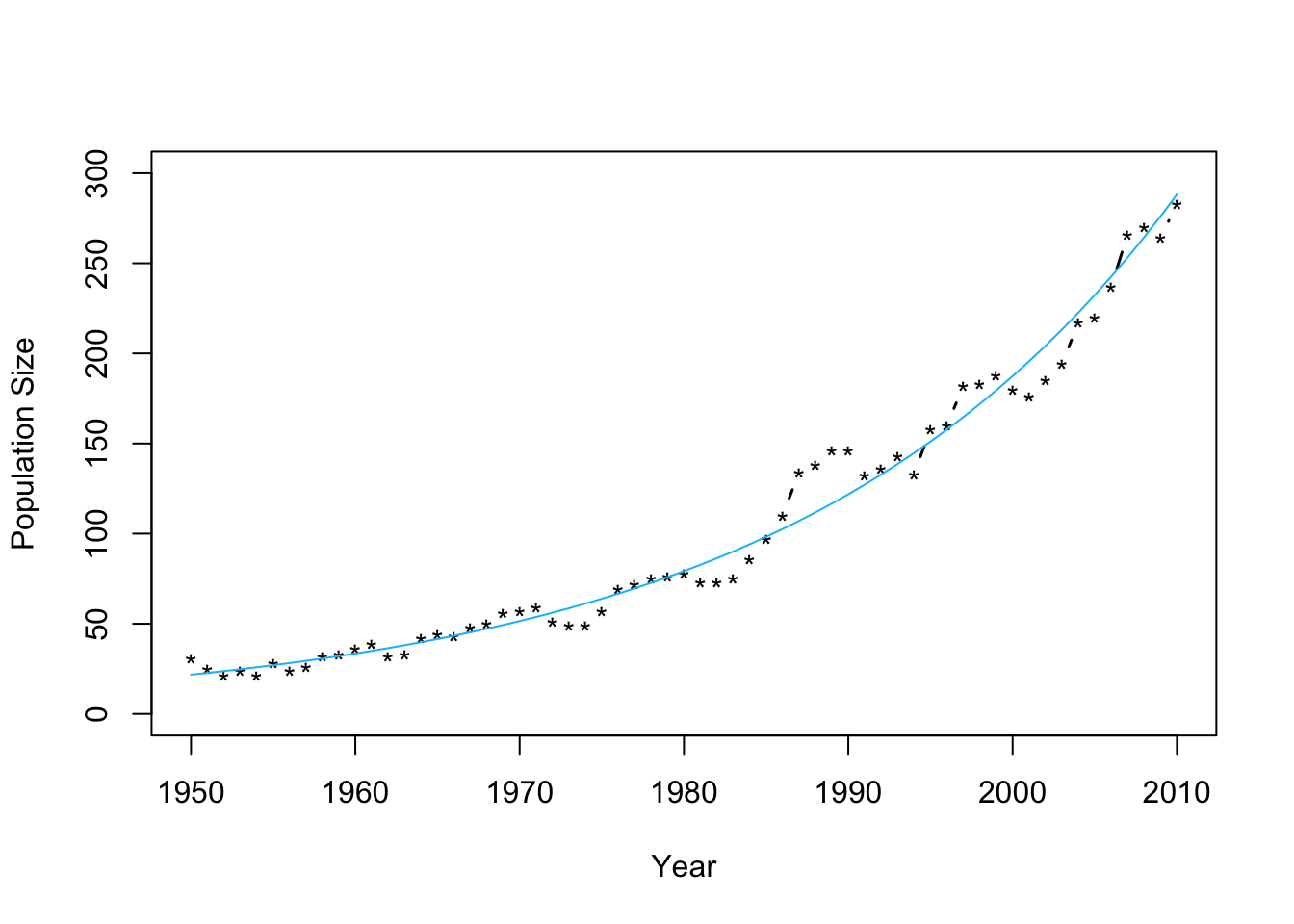
## fit lwr upr ## 1 3.080718 3.0223 3.139136## fit lwr upr ## 1 3.080718 2.842504 3.318933