Chapter 13 Tree-based Models
Tree-based models are a class of nonparametric algorithms that work by partitioning the feature space into a number of smaller (non-overlapping) regions with similar response values using a set of splitting rules.
For example, the following figures show a tree-based classification model built on two predictors.
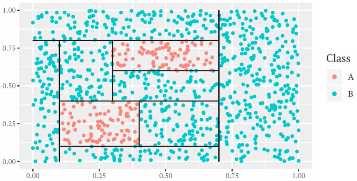
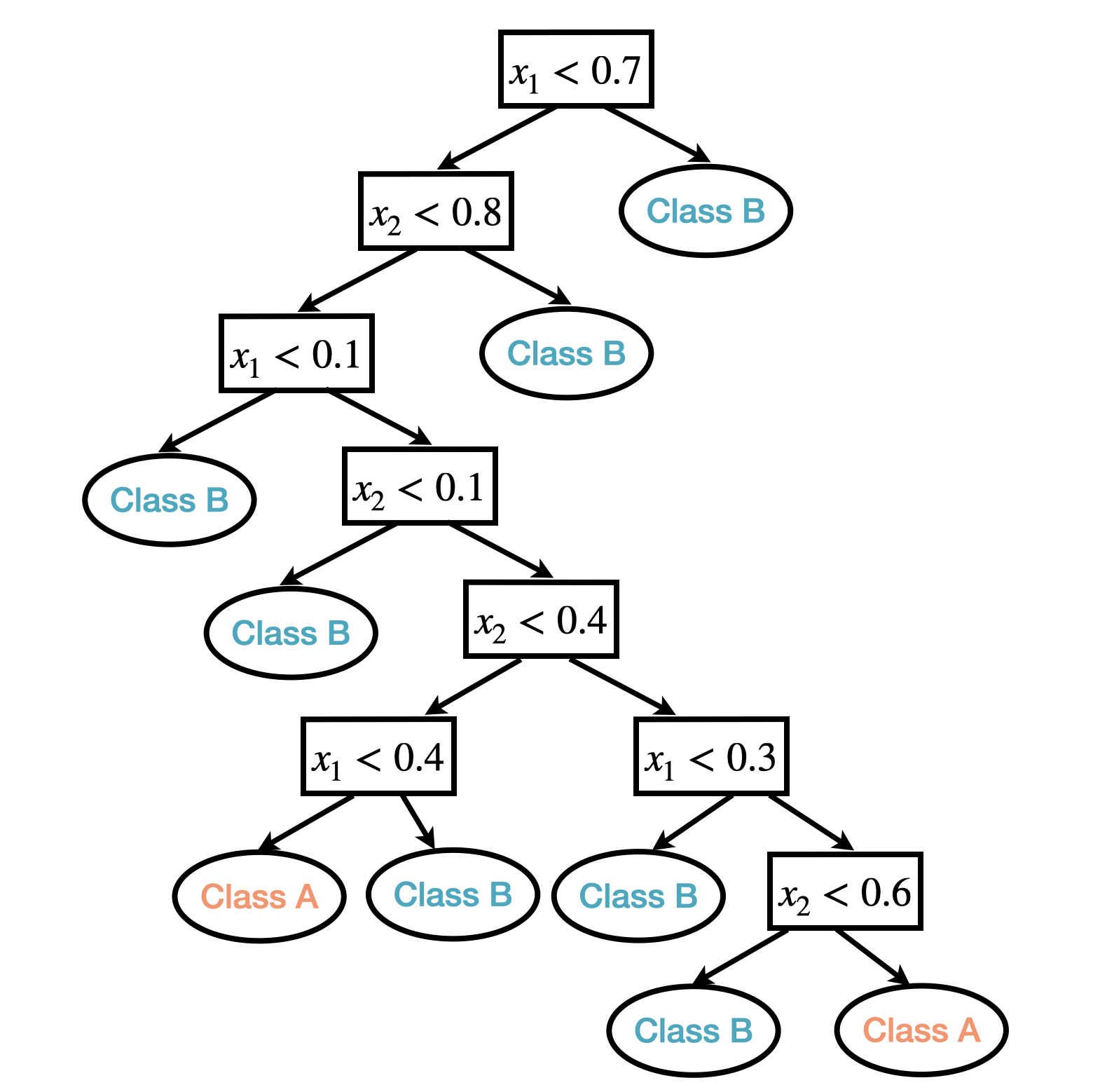
Figure 13.1: An example of classification tree based one two predictors.
Definitions
Nodes: The subgroups that are formed recursively using binary partitions formed by asking simple yes-or-no questions about each feature (e.g., \(x_1 < 0.7\)?).
We refer to the first subgroup at the top of the tree as the root node (this node contains all of the training data).
The final subgroups at the bottom of the tree are called the terminal nodes or leaves.
The rest of the subgroups are referred to as internal nodes.
The connections between nodes are called branches.
Depth of a tree is the length of the longest path from a root to a leaf.
Size of a tree is the number of terminal nodes in the tree.
In the tree model example above, there are 8 internal nodes and 9 terminal nodes; the depth of the tree is 8 and the size of the tree is 9.
As we’ll see, tree-based models offer many benefits; however, classic tree-based models, classification and regression trees, typically lack in predictive performance compared to more complex algorithms like neural networks. Fortunately, we can blend powerful ensemble algorithms into the tree-based model, for example, random forests and boosting trees, to improve the predictive performance. In this chapter, we will explore various tree-based models.
13.1 Classification and Regression Trees
There are many methodologies for constructing tree-based models, but the most well-known and classic is the classification and regression tree (CART) algorithm. A classification and regression tree partitions the training data into homogeneous subgroups (i.e., groups with similar response values) and then fits a simple constant in each subgroup. Mathematically, A classification and regression tree ends in a leaf node which corresponds to some hyper-rectangle in feature (predictor) space, \(R_j,\; j=\{1,...,J\}\), i.e. the feature space defined by \(X_1,X_2,...,X_p\) is divided into \(J\) distinct and non-overlapping regions.
- Regression tree, assigns a value to each \(R_j\), that is the model predicts the output based on the average response values for all observations that fall in that subgroup.
- Classification tree, assigns a class label to each \(R_j\), that is the model predicts the output based on the class that has majority representation or provides predicted probabilities using the proportion of each class within the subgroup.
Interpretation
Classification trees mimic some decision making processes. For example, the following decision tree is used by A&E doctors to decide what bed type to assign:
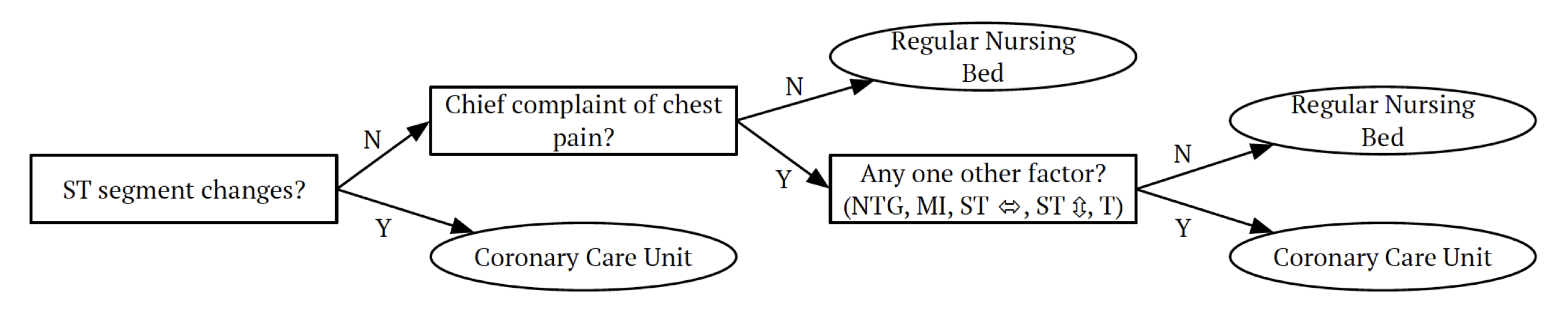
Note that trees can be constructed even in the presence of qualitative predictor variables, for example, eye colors (blue, green, brown). As tree methods can produce simple rules that are easy to interpret and visualize with tree diagrams, tree methods often refer to decision trees, which perhaps makes them popular for the feeling of interpretability and of being like a data-learned expert system.
Building trees
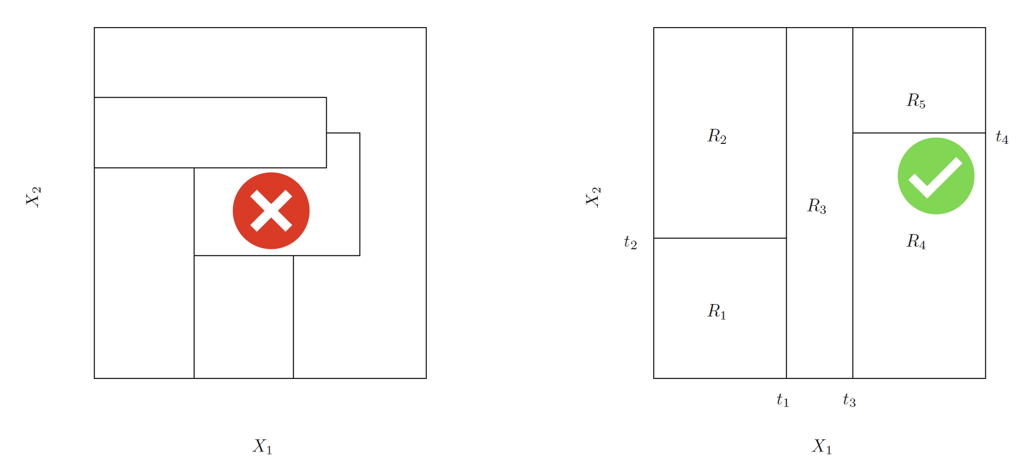
In theory, the regions \(R_j\) could have any shape. But we choose hyper (high-dimensional)-rectangles (boxes) for simplicity. The left panel is an example of an invalid partitioning, and the right is an example of a valid one.
Performance Metric
For regression trees, the goal is to find \(R_j,\; j=\{1,...,J\}\) that minimizing the RSS \[\sum_{j=1}^J\sum_{i:x_i\in R_j}(y_i-\hat{y}_{R_j})^2,\] where \(\hat{y}_{R_j}\) is the mean response for the training observations within the jth rectangle.
For classification trees, we may adopt classification error rate \(E=1-\max_k(\hat{p}_{jk})\) as performance criteria, where \(\hat{p}_{jk}\) represents the proportion of training observations in the jth region that are from the kth class. However, it turns out that the classification error rate is not sufficiently sensitive for tree-growing, especially when the data is noisy. And in practice, two other metrics are preferable:
- Gini index: \(G=\sum^K_{k=1}\hat{p}_{jk}(1-\hat{p}_{jk})\)
- Entropy: \(D=-\sum^K_{k=1}\hat{p}_{jk}\log\hat{p}_{jk}\)
Note that Both functions will take on a value near zero if the \(\hat{p}_{jk}\)’s are all near zero or near one.
Greedy fitting algorithm
It is computationally infeasible to consider every possible partition of the feature space into \(J\) boxes. Think about how many ways one could divide this 2-D space into 5 boxes. Not to mention high dimensional feature space. Therefore, in practice, we adopt the so-called Greedy(top-down) fitting algorithm:
Initialise hyper-rectangle, \(R=\mathbb{R}^d\).
Find the best (based on some objective function) split on variable \(x_i\) at location \(s\), gives \(R_1(i,s)=\{x\in R: x_i<s\}\) and \(R_2(i,s)=\{x\in R: x_i\ge s\}\).
Repeat step 2. twice, once with \(R=R_1(i,s)\) and once with \(R=R_2(i,s)\)
There will be some stopping rule, for example, requiring a minimum number (for example, 5) of training observations in each hyper-rectangle (box).
Note that such a greedy fitting algorithm does NOT guarantee an optimal tree since it is constructed stepwisely.
Pruning trees
The fitting procedure described above may produce good predictions on the training set, but is likely to overfit the data, leading to poor test set performance. To balance this trade-off between variance and bias and avoid overfitting, we often prune trees by adopting the so-called weakest link pruning algorithm in practice.
The weakest link pruning (or cost complexity pruning) introduces a nonnegative tuning parameter \(\alpha\), for regression trees minimising \[\sum_{j=1}^{|T|}\sum_{i:x_i\in R_j}(y_i-\hat{y}_{R_j})^2+\alpha|T|,\] where \(|T|\) is the number of terminal nodes (size) of the tree \(T\) (for classification trees simply replace the RSS with classification objective function, e.g. Gini index). Minimisation is achieved by attempting to remove terminal nodes from the base of the tree upward. Similar to Lasso regression, \(\alpha\) is a penalty on the size (complexity) of the tree. When \(\alpha=0\), we will keep the whole tree and when \(\alpha=\infty\), we will prune everything back to null tree (the forecast is simply the average of the response). And as always, we may Select \(\alpha\) using cross-validation.
Pros and Cons
The advantages of CART are:
Simple and easy to interpret
Akin to common decision making processes
Good visualisations
Easy to handle qualitative predictors (avoid dummy variables)
The disadvantages of CART are:
Trees tend to have high variance, small changes in the sample lead to dramatic cascading changes in the fit!
poor prediction accuracy.
Practical Demonstration
This practical demonstration will be based on synthetic (surrogate) datasets. As the name suggests, quite obviously, a synthetic dataset is a repository of data that is generated programmatically (artificially), it is not collected by any real-life survey or experiment. In practice, it is almost impossible to know the underlying system behind the real data. For synthetic data, however, we know exactly what is the underlying system behind the data. It provides a flexible and rich “test” environment to help us to explore a methodology, demonstrate its effectiveness and uncover its pros and cons by conducting experiments upon. For example, if we want to test a linear regression fitting algorithm, we may create a synthetic dataset using a linear regression model and pretend not to know the parameters of the model.
We have introduced a greedy (top-down) fitting algorithm for building classification and regression trees. Let’s create a synthetic dataset to explore the algorithm.
set.seed(212)
#set.seed() function is used to set the random generator state.
#So that the random data generated later can be reproduced using the same "seed".
data_surrogate <- data.frame(x = c(runif(200, 0, 0.4), runif(400, 0.4, 0.65), runif(300, 0.65, 1)),
                             y = c(rnorm(200, 1.5), rnorm(400, 0), rnorm(300, 2)))
In this synthetic dataset we created, \(x\) and \(y\) are paired, for the first 200 observations, \(x\) is drawn uniformly between 0 and 0.4 and \(y\) is drawn from a normal distribution with mean 1.5 and standard deviation 1; for the next 400 observations, \(x\) is drawn uniformly between 0.4 and 0.65 and \(y\) is drawn from a normal distribution with mean 0 and standard deviation 1; and for the last 300 observations, \(x\) is drawn uniformly between 0.65 and 1 and y is drawn from a normal distribution with mean 2 and standard deviation 1.
Here is a visualization of the data set.
plot(x=data_surrogate$x[1:200], y=data_surrogate$y[1:200], col='blue',
     xlab="X", ylab="Y", pch=19, xlim=c(0,1),ylim=c(-2,4))
points(x=data_surrogate$x[201:600], y=data_surrogate$y[201:600], col='red', pch=19)
points(x=data_surrogate$x[601:900], y=data_surrogate$y[601:900], col='green', pch=19)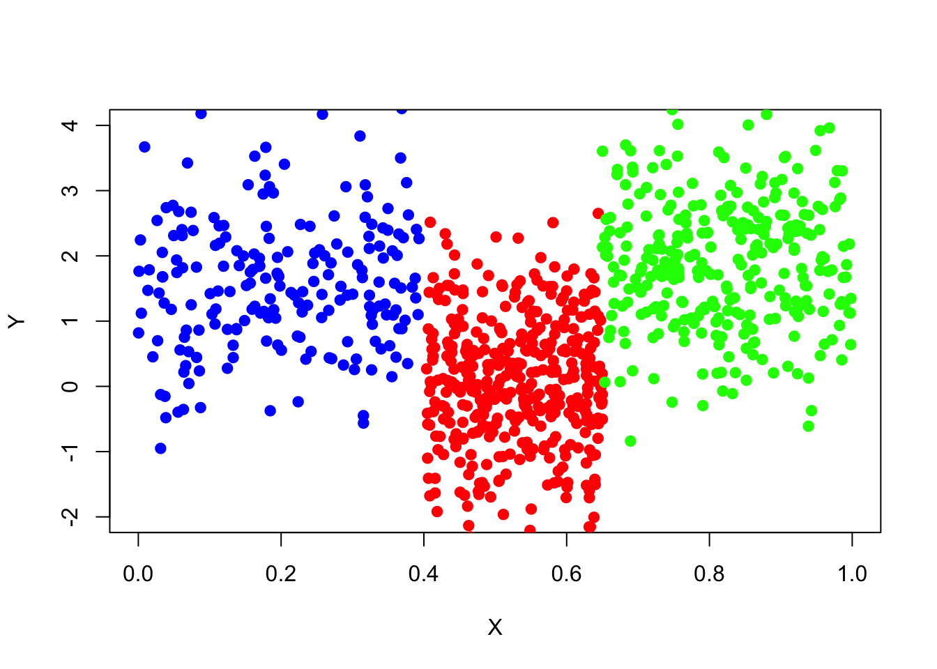
Given this data set and knowing how it was generated, the best tree-based model we would expect when modelling variable \(y\) using the variable \(x\) is a regression tree with three terminal nodes, when x is between 0 and 0.4, y equals 1.5; when x is between 0.4 and 0.65, y equals 0; x is between 0.65 and 1, y equals 2.
Now let’s build a regression tree model for this dataset using R.
library("tree")You may need to install the “tree” package first, using install.packages(“tree”).
tree_fit=tree(y~x,data_surrogate)The “tree” function is to fit a classification or regression tree using the greedy fitting algorithm.
summary(tree_fit)##
## Regression tree:
## tree(formula = y ~ x, data = data_surrogate)
## Number of terminal nodes: 3
## Residual mean deviance: 1.001 = 897.9 / 897
## Distribution of residuals:
## Min. 1st Qu. Median Mean 3rd Qu. Max.
## -3.137000 -0.662000 -0.001074 0.000000 0.638100 2.984000#The "summary" function prints a summary of the fitted tree object.
tree_fit## node), split, n, deviance, yval
## * denotes terminal node
##
## 1) root 900 1565.0 1.01200
## 2) x < 0.650076 600 883.8 0.55940
## 4) x < 0.398517 200 194.1 1.55700 *
## 5) x > 0.398517 400 391.4 0.06086 *
## 3) x > 0.650076 300 312.4 1.91700 *#print each node as well as the corresponding statisticsThe deviance is simply the residual sum of squares (RSS) for the tree/subtree.
plot(tree_fit)
text(tree_fit,pretty=0)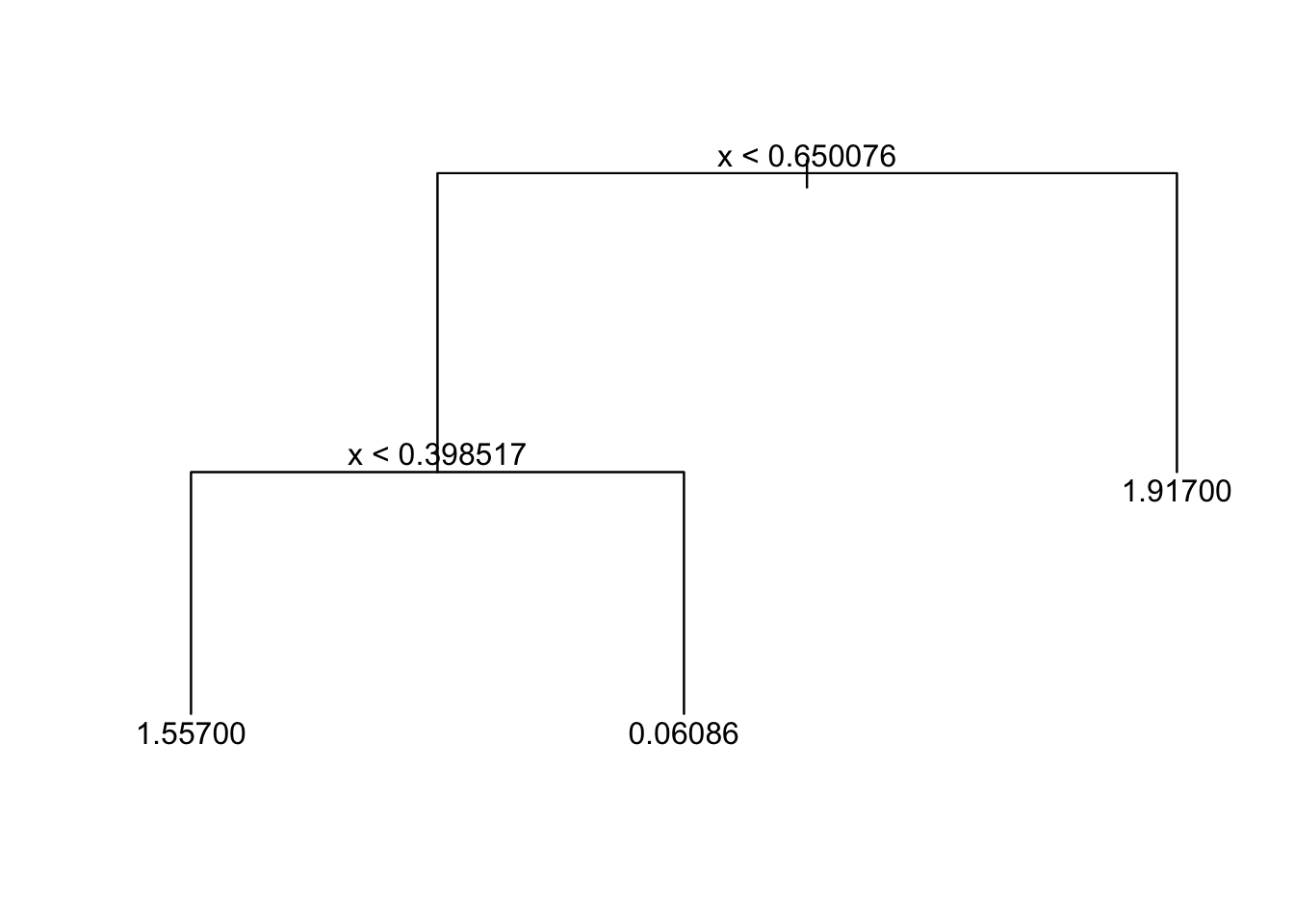
#If pretty = 0 then the level names of a factor split attributes are used unchanged. This is a nice way to plot the tree model. Is it consistent with our previous expectations?
Clearly, one of the advantages of the regression and classification tree model is its interpretation.
Now let’s examine the model performance by creating an independent data set (the same way that data_surrogate was created) as a test set, naming it data_surrogate_test and using
tree_pred=predict(tree_fit,data_surrogate_test) to generate the model prediction of y variable (in the test set) using the tree model fitted early.
set.seed(347)
data_surrogate_test <- data.frame(x = c(runif(200, 0, 0.4), runif(400, 0.4, 0.65), runif(300, 0.65, 1)),
                                  y = c(rnorm(200, 1.5),    rnorm(400, 0),         rnorm(300, 2)))
tree_pred=predict(tree_fit,data_surrogate_test)
Draw a scatter plot (same as the one drawn for data set “data_surrogate”) for the test set and add the prediction of y, “tree_pred”, to the plot. And calculate the residual sum of squares.
plot(x=data_surrogate_test$x[1:200], y=data_surrogate_test$y[1:200],
     col='blue', xlab="X", ylab="Y", pch=19, xlim=c(0,1), ylim=c(-2,4))
points(x=data_surrogate_test$x[201:600], y=data_surrogate_test$y[201:600], col='red', pch=19)
points(x=data_surrogate_test$x[601:900], y=data_surrogate_test$y[601:900], col='green', pch=19)
points(x=data_surrogate_test$x,y=tree_pred,col='black',pch=8)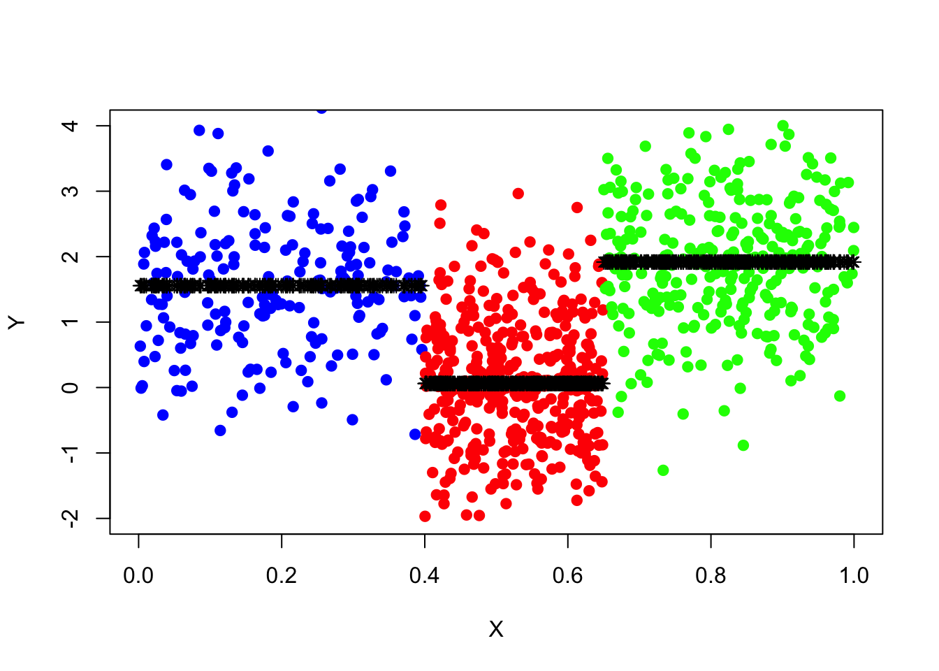
pred_mse=mean((data_surrogate_test$y-tree_pred)^2)
pred_mse
## [1] 1.005645So far, everything seems all right! The regression tree works almost perfectly. Note that we have used a rather large data set as a train set to fit the tree, what if the historical data is rather small?
Create an independent training data set (the same way that data_surrogate was created) but with the number of observations 10 times smaller. And draw a scatter plot of the data.
Then build a regression tree, name “tree_fit_s”, using the new small training set and use the new tree model to predict the y variable in the same test set data_surrogate_test and record the residual sum of squares and compare it with the one you calculated before using the tree model fitted with the large training set.
========================================================
set.seed(739)

data_surrogate_s <- data.frame(x = c(runif(20, 0, 0.4), runif(40, 0.4, 0.65),
                                     runif(30, 0.65, 1)), y = c(rnorm(20, 1.5),    rnorm(40, 0),         rnorm(30, 2)))
plot(x=data_surrogate_s$x[1:20], y=data_surrogate_s$y[1:20], col='blue',
     xlab="X", ylab="Y", pch=19, xlim=c(0,1),ylim=c(-2,4))
points(x=data_surrogate_s$x[21:60], y=data_surrogate_s$y[21:60], col='red', pch=19)
points(x=data_surrogate_s$x[61:90], y=data_surrogate_s$y[61:90], col='green', pch=19)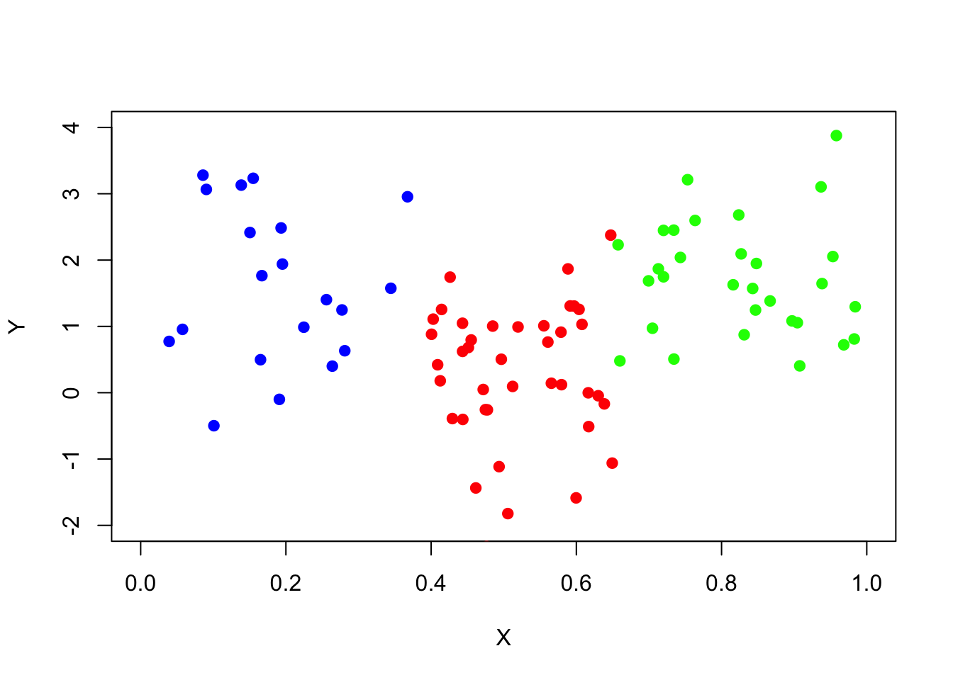
tree_fit_s=tree(y~x,data_surrogate_s)
summary(tree_fit_s)
##
## Regression tree:
## tree(formula = y ~ x, data = data_surrogate_s)
## Number of terminal nodes: 7
## Residual mean deviance: 0.89 = 73.87 / 83
## Distribution of residuals:
## Min. 1st Qu. Median Mean 3rd Qu. Max.
## -2.5420 -0.7364 0.0396 0.0000 0.5973 2.2330tree_fit_s## node), split, n, deviance, yval
## * denotes terminal node
##
## 1) root 90 131.600 1.0660
## 2) x < 0.653469 60 90.670 0.7376
## 4) x < 0.427732 26 29.650 1.4510
## 8) x < 0.160006 8 14.560 2.0450 *
## 9) x > 0.160006 18 11.020 1.1880 *
## 5) x > 0.427732 34 37.640 0.1917
## 10) x < 0.515981 16 15.670 -0.1998
## 20) x < 0.458374 6 1.973 0.3927 *
## 21) x > 0.458374 10 10.330 -0.5554 *
## 11) x > 0.515981 18 17.340 0.5398
## 22) x < 0.59835 9 2.474 0.9361 *
## 23) x > 0.59835 9 12.040 0.1435 *
## 3) x > 0.653469 30 21.480 1.7240 *plot(tree_fit_s)
text(tree_fit_s,pretty=0)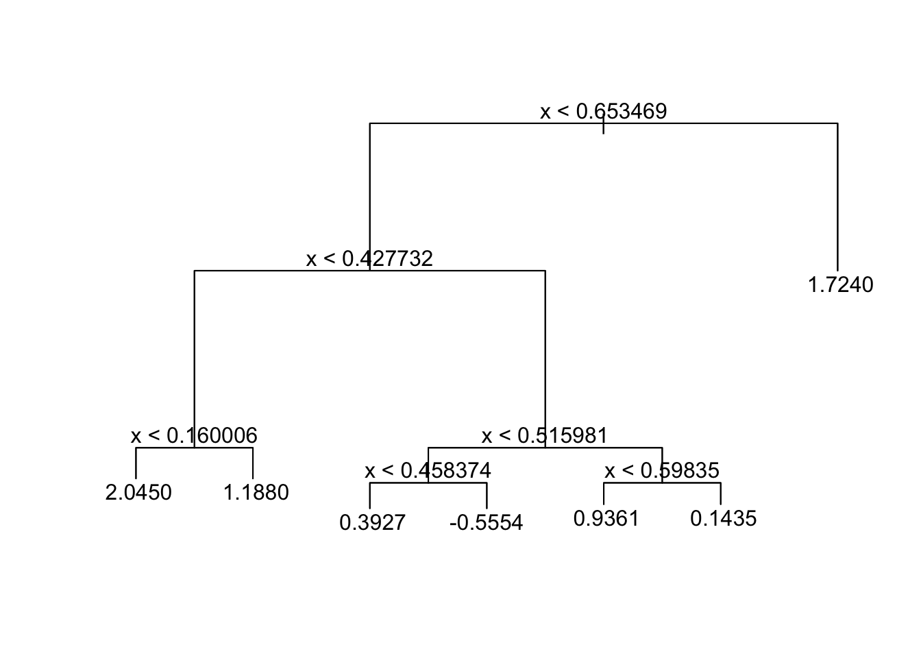
tree_pred_s=predict(tree_fit_s,data_surrogate_test)
plot(x=data_surrogate_test$x[1:200], y=data_surrogate_test$y[1:200],
     col='blue', xlab="X", ylab="Y", pch=19, xlim=c(0,1), ylim=c(-2,4))
points(x=data_surrogate_test$x[201:600], y=data_surrogate_test$y[201:600], col='red', pch=19)
points(x=data_surrogate_test$x[601:900], y=data_surrogate_test$y[601:900], col='green', pch=19)
points(x=data_surrogate_test$x,y=tree_pred_s,col='black',pch=8)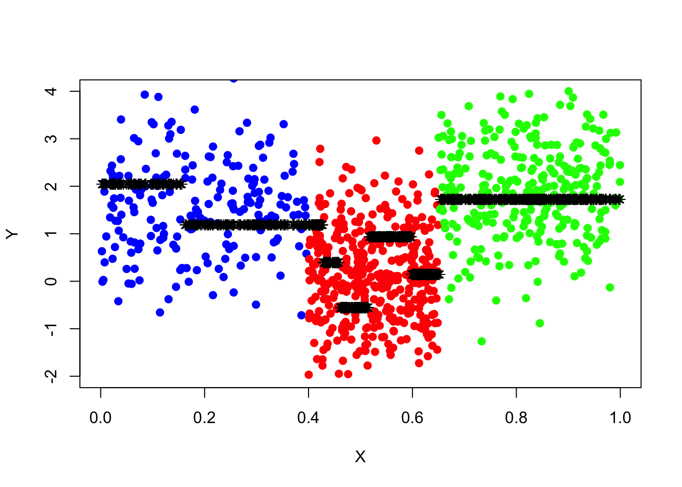
pred_mse=mean((data_surrogate_test$y-tree_pred_s)^2)
pred_mse
## [1] 1.296465The newly fitted tree, “tree_fit_s”, seems to overfit the data, which led to poor forecast performance in the test set. Now we use the cv.tree() function to see whether pruning the tree using the weakest link algorithm will improve performance.
tree_cv_prune=cv.tree(tree_fit_s,FUN=prune.tree)
tree_cv_prune
## $size
## [1] 7 6 5 4 3 1
##
## $dev
## [1] 127.1730 134.5368 127.4856 127.7807 127.2861 158.3113
##
## $k
## [1] -Inf 2.826888 3.370479 4.065974 4.633948 21.419490
##
## $method
## [1] "deviance"
##
## attr(,"class")
## [1] "prune" "tree.sequence"plot(tree_cv_prune)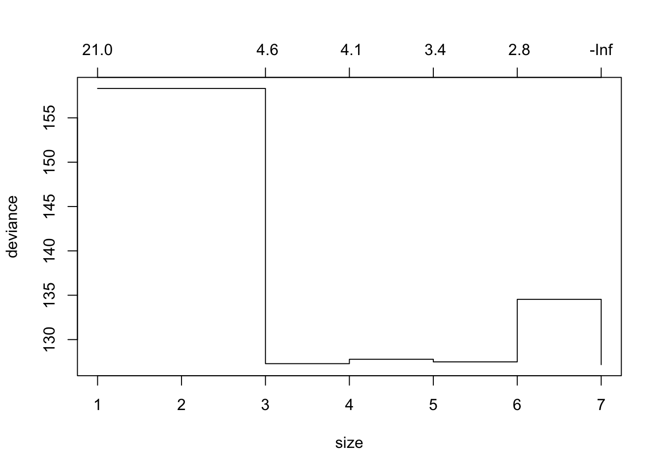
Note the output k in “tree_cv_prune” is the cost-complexity parameter in the weakest link pruning introduced in the lecture (\(\alpha\)).
tree_fit_prune=prune.tree(tree_fit_s,best=3)
# you may also prune the tree by spefifying the cost-complexity parameter k
# for example tree_fit_prune=prune.tree(tree_fit_s,k=5)
tree_fit_prune
## node), split, n, deviance, yval
## * denotes terminal node
##
## 1) root 90 131.60 1.0660
## 2) x < 0.653469 60 90.67 0.7376
## 4) x < 0.427732 26 29.65 1.4510 *
## 5) x > 0.427732 34 37.64 0.1917 *
## 3) x > 0.653469 30 21.48 1.7240 *plot(tree_fit_prune)
text(tree_fit_prune,pretty=0)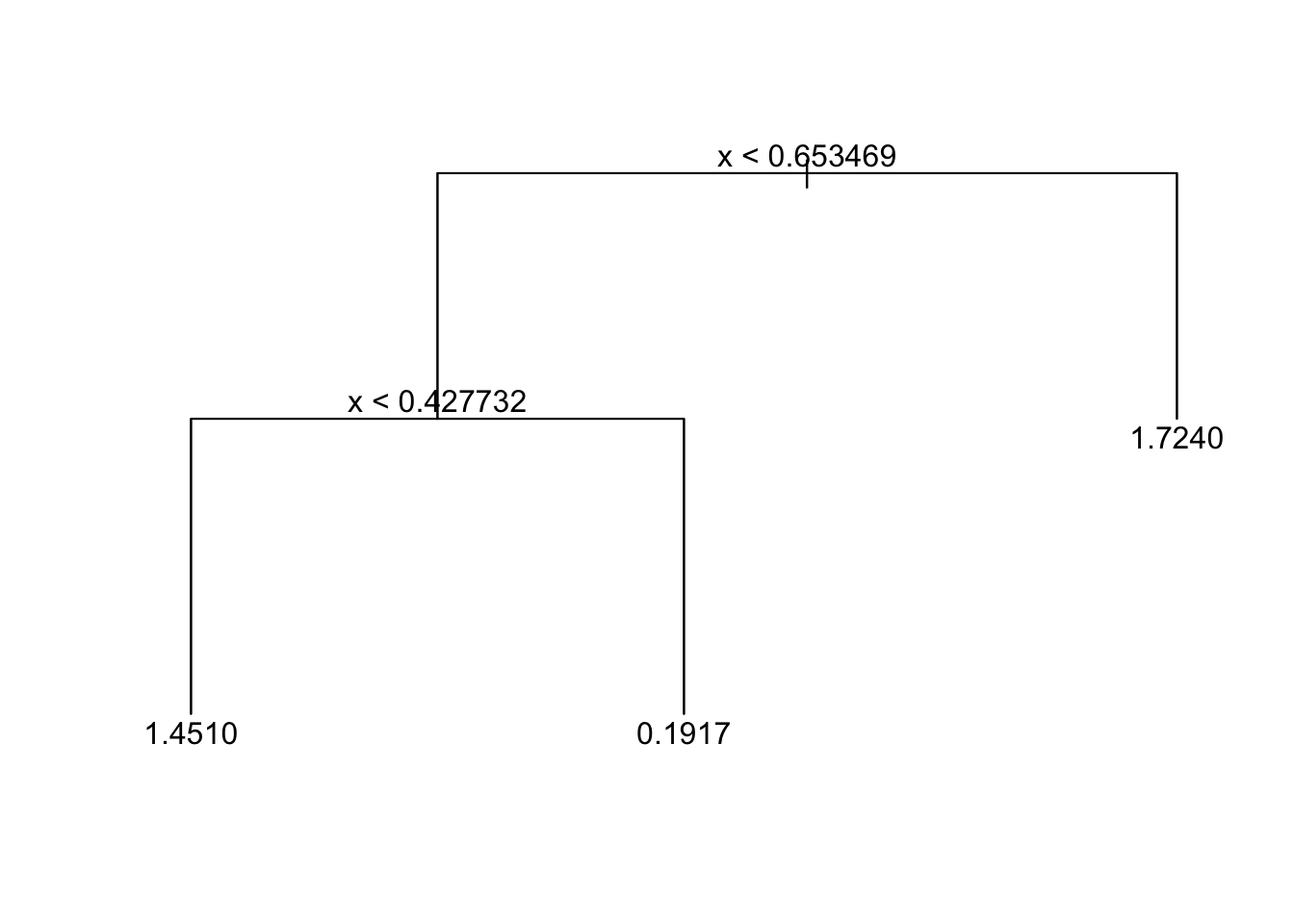
Use the pruned tree model to predict the y variable in the test set and record the mean squared error and compare the mean squared error with that resulted from an unpruned tree.
tree_pred_prune=predict(tree_fit_prune,data_surrogate_test)
plot(x=data_surrogate_test$x[1:200], y=data_surrogate_test$y[1:200],
     col='blue', xlab="X", ylab="Y", pch=19, xlim=c(0,1), ylim=c(-2,4))
points(x=data_surrogate_test$x[201:600], y=data_surrogate_test$y[201:600], col='red', pch=19)
points(x=data_surrogate_test$x[601:900], y=data_surrogate_test$y[601:900], col='green', pch=19)
points(x=data_surrogate_test$x,y=tree_pred_prune,col='black',pch=8)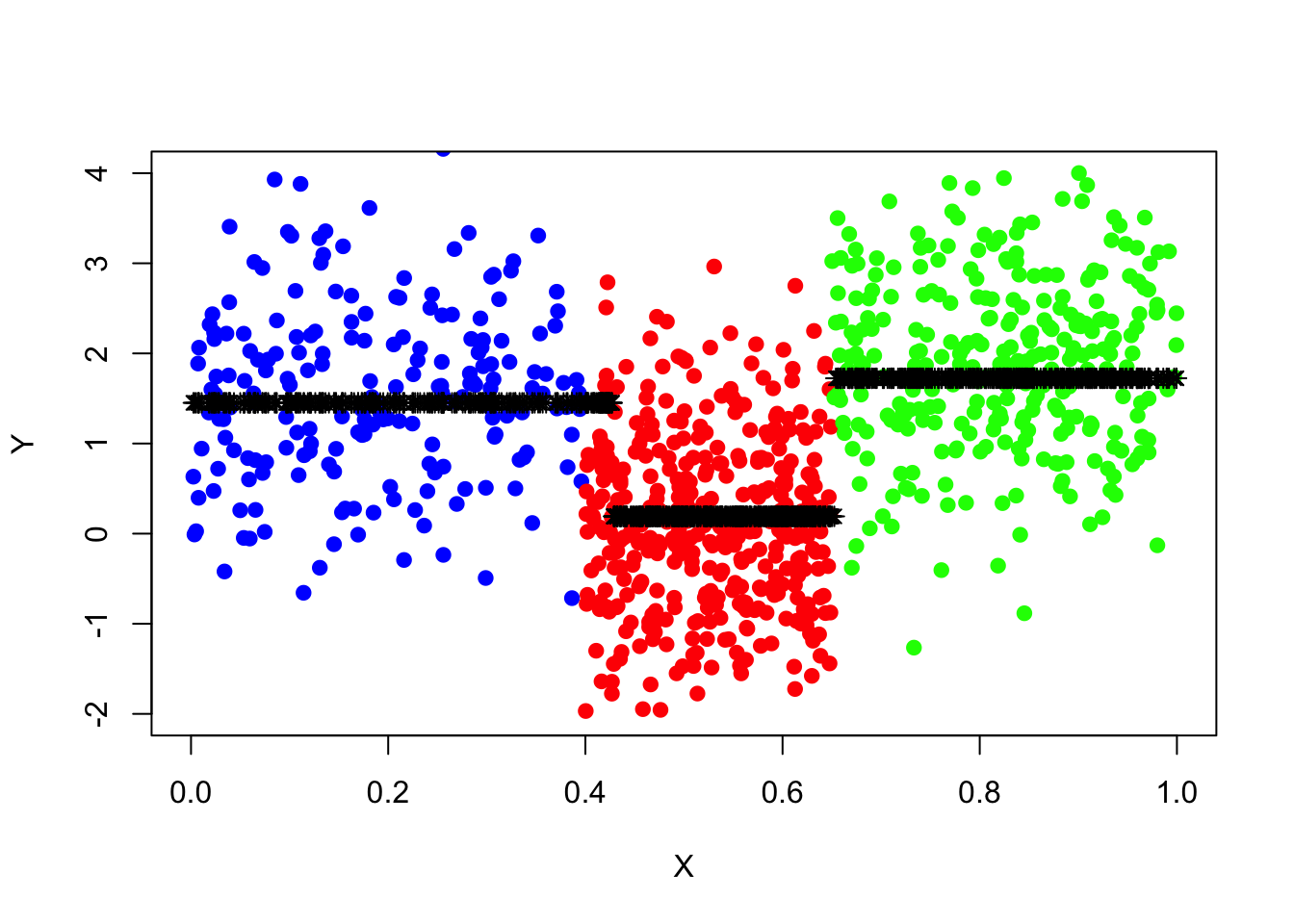
pred_mse_prune=mean((data_surrogate_test$y-tree_pred_prune)^2)
pred_mse_prune
## [1] 1.119899pred_mse-pred_mse_prune## [1] 0.1765653How would we know that the improved forecast performance is due to pruning rather than the “unlucky” small training set? To demonstrate the robustness of the conclusion, one can conduct the same experiments many times using an independent training set.
First, create a function named “prune_improvement(k)” that creates an independent small training set and compares pruned and unpruned trees with cost-complexity parameter as input parameter and returns the difference in prediction mean squared error. Then run the function 1024 times and calculate the average improvement in prediction mean squared error.
========================================================
prune_improvement <- function(k) {
  data_surrogate_s <- data.frame(x = c(runif(20, 0, 0.4), runif(40, 0.4, 0.65), runif(30, 0.65, 1)),y = c(rnorm(20, 1.5),    rnorm(40, 0),         rnorm(30, 2)))
  tree_fit_s=tree(y~x,data_surrogate_s)
  tree_pred_s=predict(tree_fit_s,data_surrogate_test)
  pred_mse_s=mean((data_surrogate_test$y-tree_pred_s)^2)
  tree_fit_prune=prune.tree(tree_fit_s,k=5)
  tree_pred_prune=predict(tree_fit_prune,data_surrogate_test)
  pred_mse_prune=mean((data_surrogate_test$y-tree_pred_prune)^2)
  dif_t=pred_mse_s-pred_mse_prune
  return(dif_t)
}
mean(sapply(1:1024, FUN=function(i){prune_improvement(5)}))
## [1] 0.0992611713.2 Bagging
We have seen CART has attractive features, but biggest problem is high variance. Bootstrap aggregating (an ensemble algorithms), also called bagging, is designed to improve the stability and accuracy of regression and classification algorithms by model averaging. Although bagging helps to reduce variance and avoid overfitting, model interpretability will be sacrificed.
Bootstrap
A bootstrap sample of size \(m\) is \((y_i^\star,\boldsymbol{x}_i^\star)^m_{i=1}\), where each \((y_i^\star,\boldsymbol{x}_i^\star)\) is a uniformly random draw from the training data \((y_1,\boldsymbol{x}_1),...,(y_n,\boldsymbol{x}_n)\). A bootstrap sample is a random sample of the data taken with replacement, which means samples in the original data set may appear more than once in the bootstrap sample. Note that when sampling from the training data \((y_1,\boldsymbol{x}_1),...,(y_n,\boldsymbol{x}_n)\) in pairs, relationship between \(y\) and \(\boldsymbol{x}\) is reserved.
There is a nice mathematical property about bootstrap samples. Let \((y_i^\star,\boldsymbol{x}_i^\star)^m_{i=1}\) are an approximation to drawing IID samples from \(\mathbb{P}(\boldsymbol{X},Y)\). If we set \(m=n\), then notionally we sampled whole new training set. However, we will only have on average \(\approx 63.2\%\) of the original training data in the bootstrap resample.
\[\begin{equation} \begin{split} \mathbb{P}(sample\; i\; is\; & in\; the\; boostrap\; resample)\\ & =1- \mathbb{P}(sample\; i\; is\;not\; in\; the\; boostrap\; resample)\\ & =1- \mathbb{P}[(\boldsymbol{x}_1^\star,y_1^\star)\neq (\boldsymbol{x}_i,y_i)\cap \dots \cap (\boldsymbol{x}_n^\star,y_n^\star)\neq (\boldsymbol{x}_i,y_i)]\\ & =1- \prod_{j=1}^{n} \mathbb{P}[(\boldsymbol{x}_j^\star,y_j^\star)\neq (\boldsymbol{x}_i,y_i)] \\ & =1-\left(1-\frac{1}{n}\right)^n \\ & \approx 1-e^{-1} \\ & \approx 0.632 \end{split} \end{equation}\]
Note that we don’t really imagine we have a new IID training sample! But bootstrap methods allow us to produce model-free estimates of sample distributions. If we have a lot of data then the estimate will be quite good. Intuitively we can roughly approximate the sampling distribution of trees for training sets of size \(n\). We then can achieve variance reduction by averaging many sampled trees.
Bagging for CART
We can apply bagging to CART in the following. For \(b=1,...,B\), draw \(n\) bootstrap samples \((y_i^\star,\boldsymbol{x}_i^\star)^n_{i=1}\) and each time fit a tree and get \(\hat{f}^{*b}(\boldsymbol{x})\), the prediction at a point \(\boldsymbol{x}\).
For regression trees, average all the predictions to obtain: \[\hat{f}^{bag}(\boldsymbol{x})=\frac{1}{B}\sum^{B}_{b=1}\hat{f}^{*b}(\boldsymbol{x})\]
For classification trees, we choose the class label for which the most bootstrapped trees “voted”. Or to construct a probabilistic prediction for \(j^{th}\) class by directly averaging tree output probabilities \[\hat{f}_j^{bag}(\boldsymbol{x})=\frac{1}{B}\sum^{B}_{b=1}\hat{f}^{*b}_j(\boldsymbol{x})\]
Bagging for CART address the overfitting issue by
Grow large trees with minimal (or no) pruning. Relies on bagging procedure directly to avoid overfit.
Prune each tree as was described in the last lecture.
Another nice property of bagging for CART is that it automatically provides out of sample evaluation. In fact, we don’t need to do cross-validation for bagging, because we know on average \(36.8\%\) of original data will NOT be in bootstrap sample so can be used as a test set. Such kind of Out Of Bag(OOB) error estimation is approximately equal to a 3-fold cross validation.
Pros and Cons
The advantages of bagging are:
If you have a lot of data, bagging is a good choice because the empirical distribution will be close to the true population distribution
Bagging is not restricted to trees, it can be used with any type of method.
It is most useful when it is desirable to reduce the variance of a predictor. Note under the (inaccurate) independence assumption, variance will be reduced by a factor of \(\sim 1/B\) for \(B\) bootstrap resamples (Central limit theorem).
Out of sample evaluation without using cross-validation, since any given observation will not be used in around \(36.8\%\) of the models.
The disadvantages of bagging are:
We lose interpretability as the final estimate is not a tree.
Computational cost is multiplied by a factor of at least \(B\).
Bagging trees are correlated, the more correlated random variables are, the less the variance reduction of their average.
13.3 Random Forests
Bagging improved on a single CART model by reducing the variance through resampling. But, in fact the bagged models are still quite correlated. And the more correlated random variables are, the less the variance reduction of their average. Can we make them more independent in order to produce a better variance reduction? Random forecasts achieve this by not only resampling observations, but by restricting the model to random subspaces, \(\mathcal{X}'\subset \mathcal{X}\).
Methodology
The Random Forests algorithm can be implemented in the following:
Take a bootstrap resample \((y_i^\star,\boldsymbol{x}_i^\star)^n_{i=1}\) of the training data as for bagging.
Building a tree, each time a split in a tree is considered, random select \(m\) predictors out of the full set of \(p\) predictors as split candidates, and find the “optimal” split within those \(m\) predictors. (typically choose \(m\approx \sqrt{p}\))
Repeat 1) and 2), average the prediction of all trees.
Interpretation
Classification and regression trees are easy to interpret and follow common human decision making mechanisms. Linear models provides statistical significance tests (e.g. t-test, z-test of parameter significance). Random Forecasts may seem great, but we’ve sacrificed interpretability with bagging and random subspace. There are two popular approaches that can help us to quantify the importance of each variable.
For each feature variable \(x_{j}, \;j=1,…,p\), loop over each tree in the forest,
- find all nodes that make a split on \(x_{j}\)
- compute the improvement in loss criterion the split causes (e.g. accuracy/Gini/etc)
- sum improvements across nodes in the tree
Finally, sum improvement across all tress.
We already discussed that bagging enables out of bag error estimate. We can then compute out of bag variable importance for each feature \(x_{j},\; j=1,…,p\) in the following:
- For each tree, take the out of bag samples data matrix, \(\boldsymbol{x}^{oob}\), and compute the predictive accuracy for that tree;
- Take \(\boldsymbol{x}^{oob}\) and randomly permute all the entries \(j^{th}\) column (break the ties between \(x_j\) and the rest of variables);
- Pass the modified \(\boldsymbol{x}^{oob^*}\) through the tree and compute the change in predictive accuracy for that tree.
Finally average the decrease in accuracy over all trees.
Pros and Cons
The advantages of random forests are:
- Inherits the advantages of bagging and trees
- Very easy to parallelise
- Works well with high dimensional data
- Tuning is rarely needed (easy to get good quality forecast)
The disadvantages of random forests are:
- Often quite suboptimal for regression.
- Same extrapolation issue as trees.
- Harder to implement and memory hungry model.
13.4 Boosting
Boosting is an extremely popular machine learning algorithm that has proven successful across many domains and is one of the leading methods for winning Kaggle competitions. Whereas random forests build an ensemble of deep independent trees, Boosting builds an ensemble of shallow trees in sequence with each tree learning and improving on the previous one. Although shallow trees by themselves are rather weak predictive models, they can be “boosted” to produce a powerful “committee” that, when appropriately tuned, is often hard to beat with other algorithms.
Methodology Boosting is similar to bagging in the sense that we combine results from multiple classifiers, but it is fundamentally different in approach:
Set \(\hat{f}(\boldsymbol{x})=0\) and \(\epsilon_i=y_i\) for \(i=1,…,n\).
For \(b=1,…,B\), iterate:
- Fit a model (eg tree) \(\hat{f}^b(\boldsymbol{x})\) to the response \(\epsilon_1,…,\epsilon_n\)
- Update the predictive model to \[\hat{f}(\boldsymbol{x}) \leftarrow \hat{f}(\boldsymbol{x}) + \lambda \hat{f}^b(\boldsymbol{x}) \]
- Update the residuals \[ \epsilon_i \leftarrow \epsilon_i-\lambda\hat{f}^b(\boldsymbol{x}) \;\;\;\; \forall i\]
Output as final boosted model \[\hat{f}(\boldsymbol{x}) =\sum^B_{b=1}\lambda \hat{f}^b(\boldsymbol{x}) \]
Intuitively Boosting is a
Slow learning approach: Aim to learn usually simple model (which leads to low variance, but high bias) in each round. Then bring bias down by repeating over many rounds.
Sequential learning: Each round of boosting aims to correct the error of the previous rounds.
Generic methodology: Any model at all can be boosted! Completely general method.
Tuning parameters for boosting
There are three main hyper-parameters that need to be tuned for building boosting tree model.
The number of trees \(B\). Unlike bagging and random forests, boosting can overfit if \(B\) is too large, although this overfitting tends to occur slowly if at all. We use cross-validation to select \(B\).
The shrinkage parameter \(\lambda\), a small positive number. This controls the rate at which boosting learns. Typical values are 0.01 or 0.001, and the right choice can depend on the problem. Very small \(\lambda\) can require using a very large value of \(B\) in order to achieve good performance.
The number of splits \(d\) in each tree, which controls the complexity of the boosted ensemble. Often \(d=1\) works well, in which case each tree consists of a single split and resulting in an additive model. More generally \(d\) is the interaction depth, and controls the interaction order of the boosted model, since \(d\) splits can involve at most \(d\) variables.
Boosting discussion Boosting is an incredibly powerful technique and regularly is instrumental in winning machine learning competitions. Any model at all can be boosted. However, tuning is needed (not trivial) and some difficulties in interpretation and extrapolation.
13.5 Practical Demonstration
We now explore all the tree-based model by analyzing the Boston housing data. The goal is to build a model to predict variable medv using the rest of variables.
library(ISLR)
library(tree)
library(MASS)
We first divide the dataset into two part, training set (half the dataset) and test set (the other half the dataset).
set.seed (1)
train = sample (1: nrow(Boston ), nrow(Boston )/2)
data_train=Boston[train,]
data_test=Boston[-train,]
Fit a regression tree to the training set, plot the tree.
tree.boston=tree(medv~.,data_train)
summary(tree.boston)
##
## Regression tree:
## tree(formula = medv ~ ., data = data_train)
## Variables actually used in tree construction:
## [1] "rm" "lstat" "crim" "age"
## Number of terminal nodes: 7
## Residual mean deviance: 10.38 = 2555 / 246
## Distribution of residuals:
## Min. 1st Qu. Median Mean 3rd Qu. Max.
## -10.1800 -1.7770 -0.1775 0.0000 1.9230 16.5800plot(tree.boston)
text(tree.boston,pretty =0)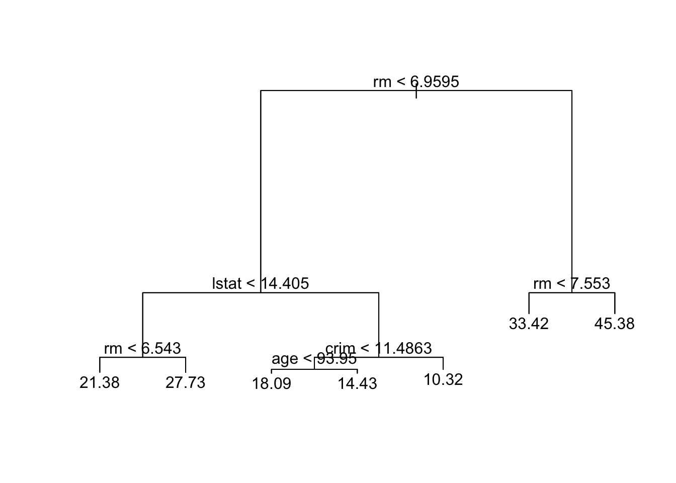
Predict medv using the test set and record the mean squared error.
yhat=predict(tree.boston,data_test)
mean((yhat -data_test$medv)^2)
## [1] 35.28688Prune the tree using cv.tree() and plot the pruned tree
cv.boston =cv.tree(tree.boston)
plot(cv.boston)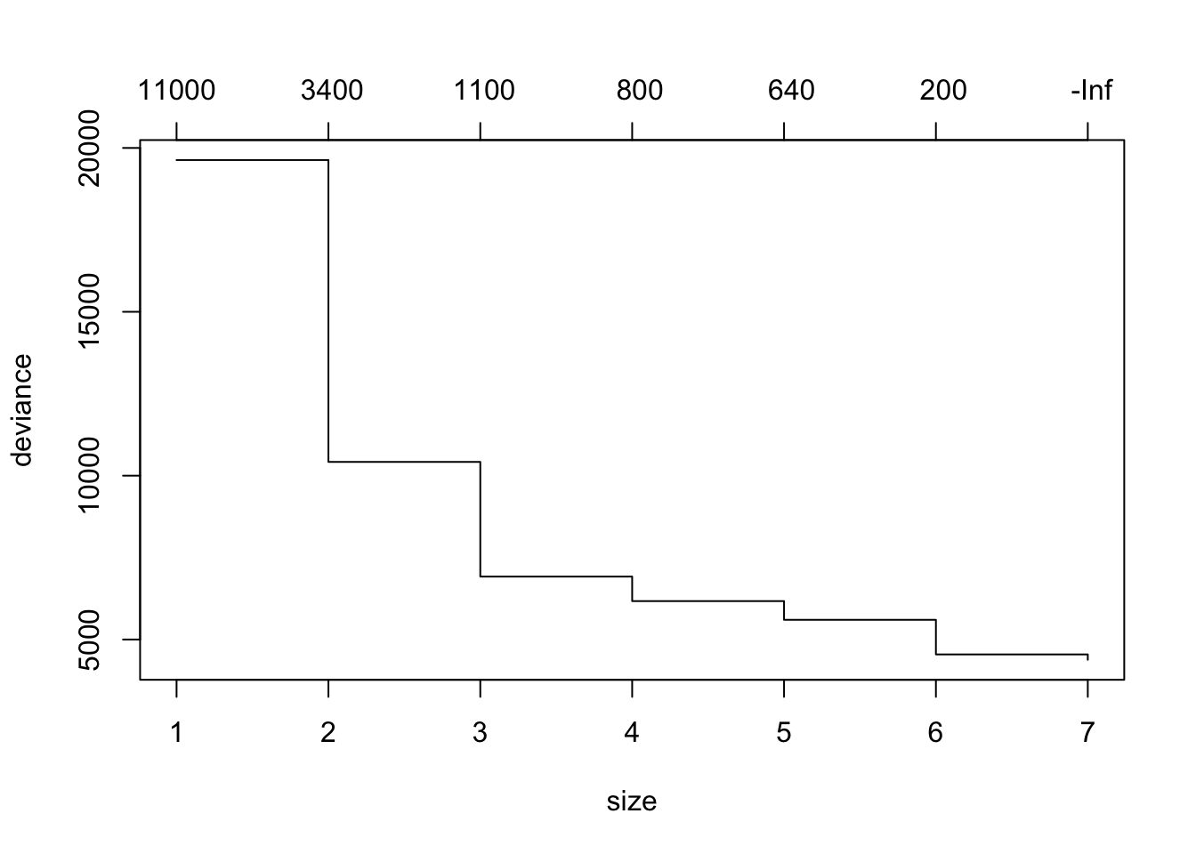
prune.boston =prune.tree(tree.boston ,best =6)
plot(prune.boston)
text(prune.boston,pretty =0)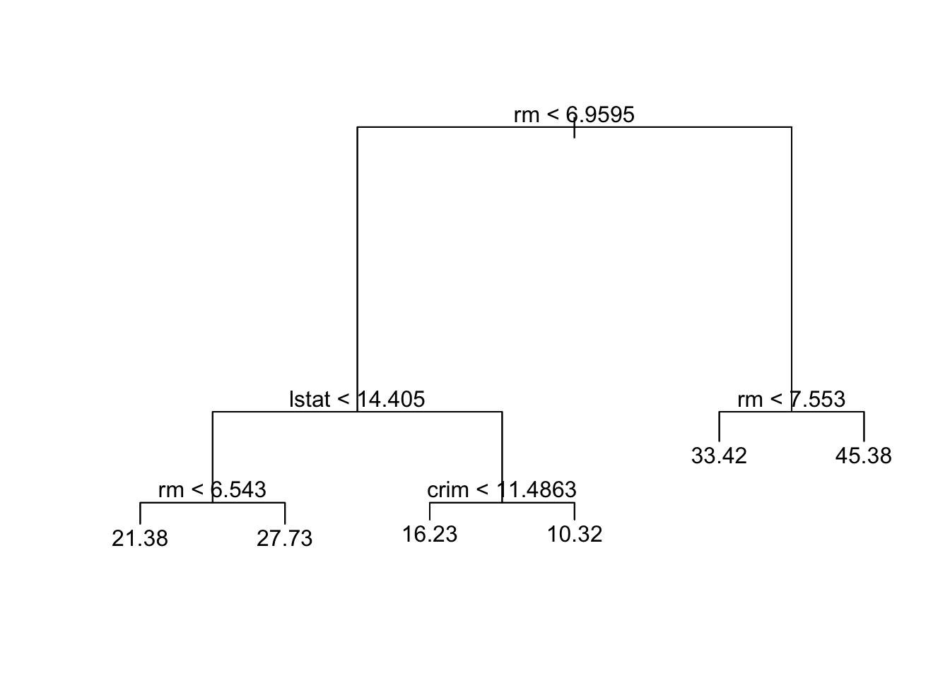
Predict medv using the test set and pruned tree, recorder the mean squared error and compare it with unpruned tree.
yhat=predict(prune.boston,data_test)
mean((yhat -data_test$medv)^2)
## [1] 35.16439Here we apply bagging and random forests to the Boston data, using the randomForest package in R. Note that bagging is simply a special case of a random forest with m = p. Therefore, the randomForest() function can be used to perform both random forests and bagging. We perform bagging as follows:
library (randomForest)## randomForest 4.6-14## Type rfNews() to see new features/changes/bug fixes.##
## Attaching package: 'randomForest'## The following object is masked from 'package:ggplot2':
##
## margin#you may need to install the randomForest library first
set.seed (472)
bag.boston =randomForest(medv~.,data=data_train,mtry=13, ntree=10, importance =TRUE)## Warning in randomForest.default(m, y, ...): invalid mtry: reset to within valid
## rangebag.boston##
## Call:
## randomForest(formula = medv ~ ., data = data_train, mtry = 13, ntree = 10, importance = TRUE)
## Type of random forest: regression
## Number of trees: 10
## No. of variables tried at each split: 12
##
## Mean of squared residuals: 13.45607
## % Var explained: 82.49Note there are 13 predictors in the Boston data, the argument mtry=13 indicates that all 13 predictors are considered for each split of the tree, in other words, bagging is conducted. ntree=10 indicates 10 bootstrap trees are generated in this bagged model. The MSR and % variance explained are based on OOB (out-of-bag) estimates
We can also evaluate the performance of bagged model using the test set:
pred.bag = predict (bag.boston,newdata =data_test)
plot(pred.bag , data_test$medv)
abline (0,1)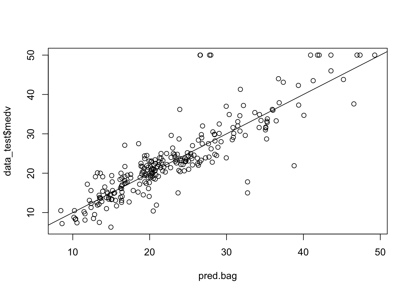
mean(( pred.bag -data_test$medv)^2)## [1] 22.44938The test set MSE associated with the bagged regression tree is much smaller than that obtained using an optimally-pruned single CART.
We now Increase the number of bootstrap trees generated in the bagged model to 100 and 1000, record the test set MSE respectively and compare them to the bagged model with 10 bootstrap trees.
bag.boston =randomForest(medv~.,data=data_train,mtry=13, ntree=100, importance =TRUE)## Warning in randomForest.default(m, y, ...): invalid mtry: reset to within valid
## rangepred.bag = predict (bag.boston,newdata =data_test)
mean(( pred.bag -data_test$medv)^2)## [1] 23.13702bag.boston =randomForest(medv~.,data=data_train,mtry=13, ntree=1000, importance =TRUE)## Warning in randomForest.default(m, y, ...): invalid mtry: reset to within valid
## rangepred.bag = predict (bag.boston,newdata =data_test)
mean(( pred.bag -data_test$medv)^2)## [1] 23.54552We now Grow a random forest proceeds in exactly the same way, except that we use a smaller value of the mtry argument. By default, randomForest() uses \(p/3\) variables when building a random forest of regression trees, we may also try \(\sqrt{p}\) variables when building a random forest of classification trees.
rf.boston =randomForest(medv~.,data=data_train,mtry=4, ntree=100, importance =TRUE)
pred.rf = predict (rf.boston,newdata =data_test)
mean(( pred.rf -data_test$medv)^2)
## [1] 20.41462To view the importance of each variable, apply the importance() function. (type ?importance in the console for detailed description of importance() function) And use the varImpPlot() to plot the importance measures and interpret the results.
importance(rf.boston)## %IncMSE IncNodePurity
## crim 8.8561695 1236.90238
## zn 1.5940368 150.70830
## indus 4.2096189 850.89234
## chas 0.3066732 24.94713
## nox 5.8090684 881.53719
## rm 16.7918585 8110.68177
## age 5.9184141 771.57077
## dis 3.4916527 824.61307
## rad 2.5007048 203.89994
## tax 4.7607576 664.49261
## ptratio 3.3599677 1250.70664
## lstat 10.0709051 4496.94612varImpPlot(rf.boston)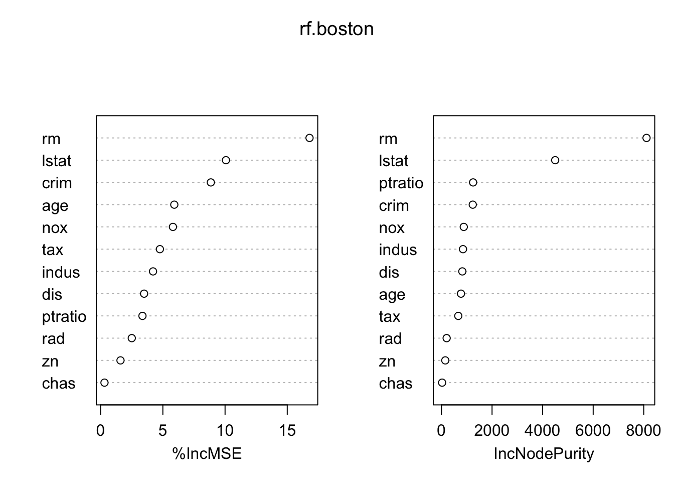
We can write a for loop to record the test set prediction MSE for all 13 possible values of mtry.
test.err=double(13)
for(mtry_t in 1:13){
  fit=randomForest(medv~.,data=data_train,mtry=mtry_t,ntree=100)
  pred=predict(fit,data_test)
  test.err[mtry_t]=mean(( pred -data_test$medv)^2)
}
## Warning in randomForest.default(m, y, ...): invalid mtry: reset to within valid
## rangeplot(test.err)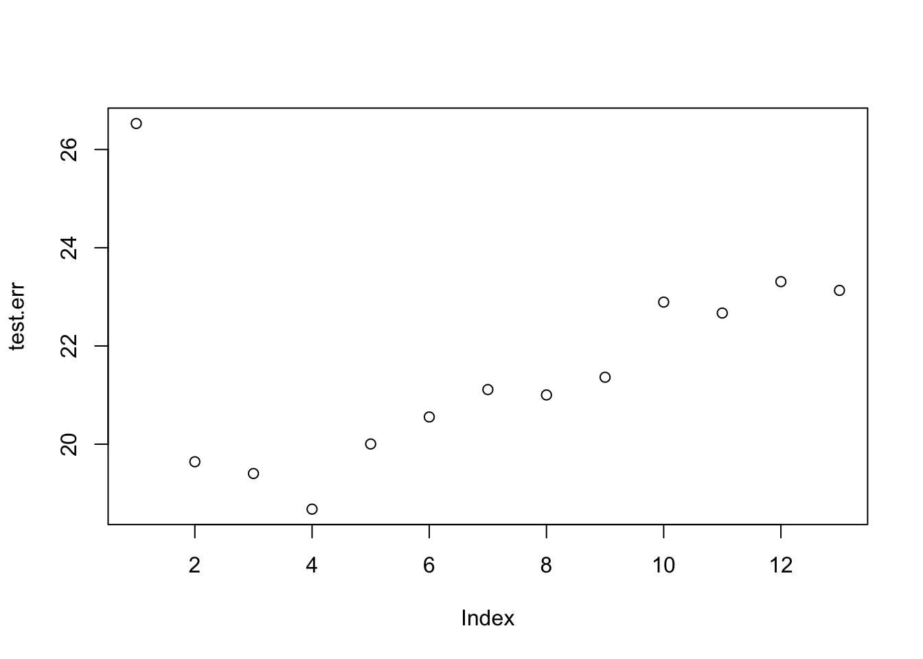
We now use the gbm package, and within it the gbm() function, to fit boosted regression trees to the Boston data set.
library (gbm)## Loaded gbm 2.1.8set.seed (517)
boost.boston =gbm(medv~.,data=data_train, distribution="gaussian",
n.trees =1000, interaction.depth =2)
summary(boost.boston)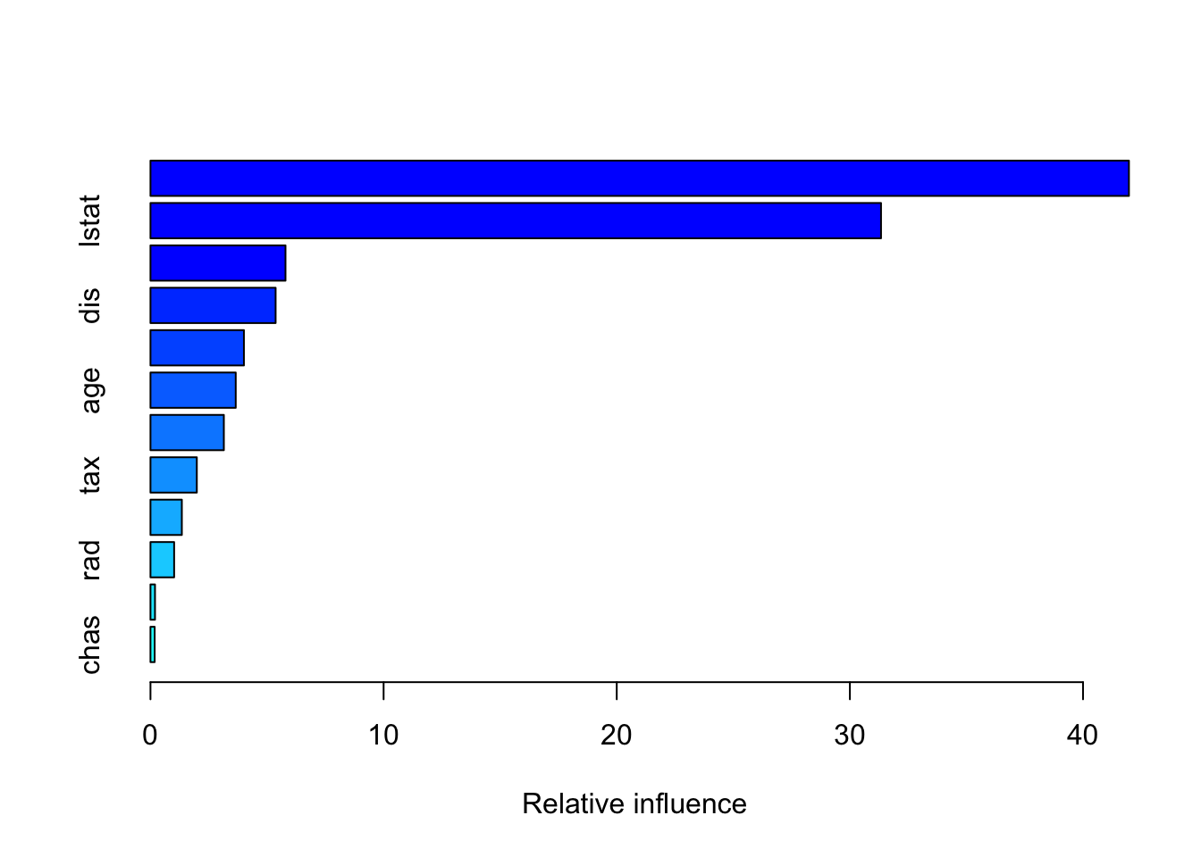
##             var    rel.inf
## rm           rm 41.9696443
## lstat     lstat 31.3357911
## crim       crim  5.7915015
## dis         dis  5.3682171
## nox         nox  4.0082986
## age         age  3.6575000
## ptratio ptratio  3.1472612
## tax         tax  1.9878973
## indus     indus  1.3455310
## rad         rad  1.0149034
## zn           zn  0.1938735
## chas       chas  0.1795809
You may look up the function gbm via ?gbm. The option distribution=“gaussian” since this is a regression problem; if it were a binary classification problem, we would use distribution=“bernoulli”. The argument n.trees=1000 indicates that we want 1000 trees, and the option interaction.depth=2 specifies the number of splits performed on each tree. The summary() function produces a relative influence plot and also outputs the relative influence statistics.
We now use the boosted model to predict medv on the test set, and record MSE. Note the boosted model outperfom random forests model built early.
pred.boost=predict(boost.boston,newdata =data_test, n.trees =1000)
mean((pred.boost-data_test$medv)^2)
## [1] 15.91325The default shrinkage parameter lambda is 0.001. We can specify its value by adding argument shrinkage in the gbm() function, for example shrinkage=0.05.