Chapter 9 Step Functions

9.1 Step Functions

Step functions use cut-points \(c_1, c_2, \ldots, c_K\) in the range of X in order to construct \(K+1\) dummy variables in the following way: \[\begin{align*} C_0(X) & = I(X \leq c_1)\\ C_1(X) & = I(c_1 < X \leq c_2)\\ & ~ ~ \vdots \\ C_{K-1}(X) & = I(c_{K-1} < X \leq c_K)\\ C_K(X) & = I(c_K < X) \end{align*}\] Above \(I(\cdot)\) is the indicator function. For example \(I(c_1 < X \leq c_2)=1\) if \(c_1 < X \leq c_2\) and equals 0 otherwise.

Note: trivially we have that: \(C_0(X) + C_1(X) + \ldots + C_K(X) = 1\) since X must be in exactly one of the \(K+1\) intervals.

After defining appropriate intervals and constructing the corresponding dummy variables we fit LS to the following model: \[ y = f(x) = \beta_0 + \beta_1 C_1(x) + \beta_2 C_2(x) + \ldots + \beta_K C_K(x) + \epsilon. \] Inclusion of \(C_0(x)\) is not needed because this effect is represented by \(\beta_0\).

This means that if \(X\leq c_1\) our prediction is \(\beta_0\), while if \(c_{j}<X\leq c_{j+1}\) we predict \(\beta_0 + \beta_j\) for \(j = 1, \ldots, K\). In other words, \(\beta_0\) can be interpreted as the mean value of \(Y\) for \(X \leq c_1\), and \(\beta_j\) represents the average increase in the response for \(X\) in \(c_j< X \leq c_{j+1}\) relative to \(X \leq c_1\).

Example: Wage Data

We apply step-function regression to model the Wage data introduced in Section 8.2, with different numbers of step functions (Figure 9.1. We can see that this modelling approach is local: new samples within a sampling interval affect only the predicted effect within that interval. We see that this approach creates a bumpy fit to the data. This is desirable sometimes in applications in biomedicine or social sciences where the goal is to report overall summaries within specific age groups. In other applications smoothness is preferable.

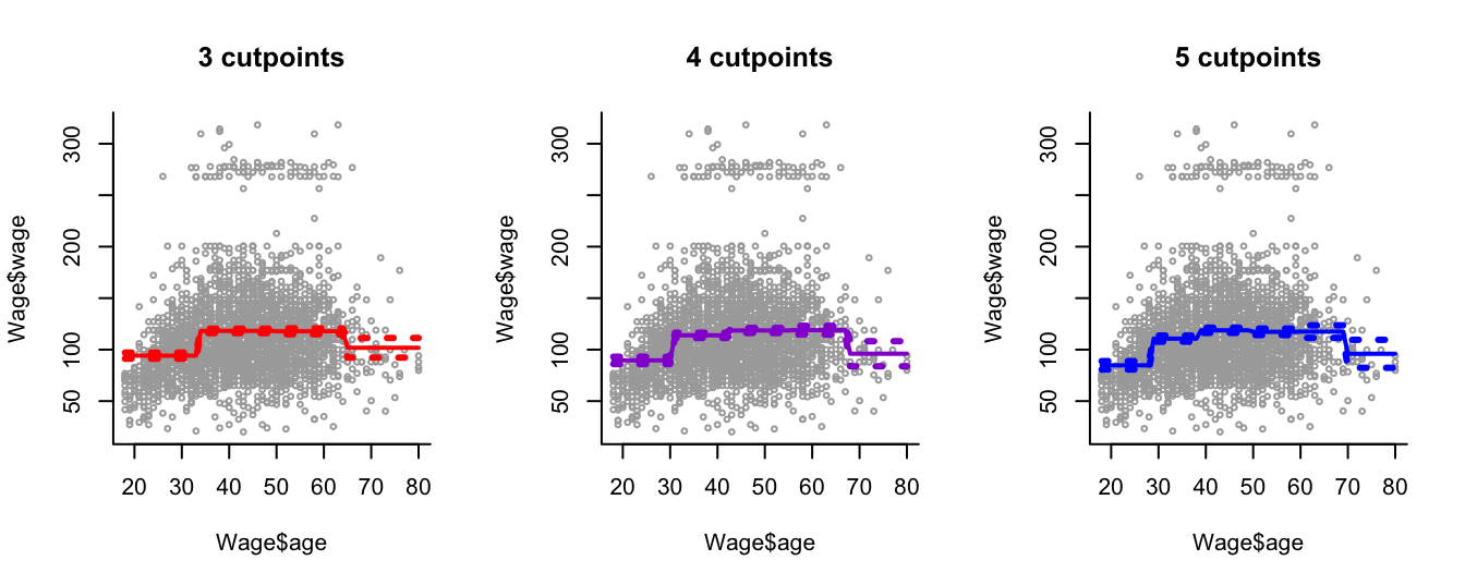
Figure 9.1: Step function regression with different numbers of cutpoints applied to the Wage data.

9.2 Practical Demonstration

We once again make use of the Boston dataset in library MASS.

library("MASS")
y = Boston$medv
x = Boston$lstat
y.lab = 'Median Property Value'
x.lab = 'Lower Status (%)'

For step function regression we can make use of the command cut(), which automatically assigns samples to intervals given a specific number of intervals. We can check how this works by executing the following line of code.

table(cut(x, 2))

## 
## (1.69,19.9]   (19.9,38] 
##         430          76

What we see is that cut(x, 2) automatically created a factor with two levels, corresponding to the intervals \((1.69, 19.9]\) and \((19.9, 38]\), and assigned each entry in \(x\) to one of these factors depending on which interval it was in. The command table() tells us that 430 samples of x fall within the first interval and that 76 samples fall within the second interval. Note that cut(x, 2) generated 2 intervals, but this means there is only 1 cutpoint (at \(19.9\)). The number of cutpoints is naturally one less than the number of intervals, but it is important to be aware that cut requires specification of the number of required intervals.

So, we can use cut() within lm() to easily fit regression models with step functions. Below we consider 4 models with 1, 2, 3 and 4 cutpoints (2, 3, 4 and 5 intervals) respectively.

step2 = lm(y ~ cut(x, 2))
step3 = lm(y ~ cut(x, 3))
step4 = lm(y ~ cut(x, 4))
step5 = lm(y ~ cut(x, 5))

The analysis then is essentially the same as previously. The following code produces the 2 by 2 plot of the fitted lines of the four models, along with approximate 95% confidence intervals for the mean predictions.

pred2 = predict(step2, newdata = list(x = sort(x)), se = TRUE)
pred3 = predict(step3, newdata = list(x = sort(x)), se = TRUE)
pred4 = predict(step4, newdata = list(x = sort(x)), se = TRUE)
pred5 = predict(step5, newdata = list(x = sort(x)), se = TRUE)

se.bands2 = cbind(pred2$fit + 2*pred2$se.fit, pred2$fit-2*pred2$se.fit)
se.bands3 = cbind(pred3$fit + 2*pred3$se.fit, pred3$fit-2*pred3$se.fit)
se.bands4 = cbind(pred4$fit + 2*pred4$se.fit, pred4$fit-2*pred4$se.fit)
se.bands5 = cbind(pred5$fit + 2*pred5$se.fit, pred5$fit-2*pred5$se.fit)

par(mfrow = c(2,2))

plot(x, y, cex.lab = 1.1, col="darkgrey", xlab = x.lab, ylab = y.lab,
     main = "1 cutpoint", bty = 'l')
lines(sort(x), pred2$fit, lwd = 2, col = "red")
matlines(sort(x), se.bands2, lwd = 1.4, col = "red", lty = 3)

plot(x, y, cex.lab = 1.1, col="darkgrey", xlab = x.lab, ylab = y.lab,
     main = "2 cutpoints", bty = 'l')
lines(sort(x), pred3$fit, lwd = 2, col = "darkviolet")
matlines(sort(x), se.bands3, lwd = 1.4, col = "darkviolet", lty = 3)

plot(x, y, cex.lab = 1.1, col="darkgrey", xlab = x.lab, ylab = y.lab,
     main = "3 cutpoints", bty = 'l')
lines(sort(x), pred4$fit, lwd = 2, col = "blue")
matlines(sort(x), se.bands4, lwd = 1.4, col = "blue", lty = 3)

plot(x, y, cex.lab = 1.1, col="darkgrey", xlab = x.lab, ylab = y.lab,
     main = "4 cutpoints", bty = 'l')
lines(sort(x), pred5$fit, lwd = 2, col = "black")
matlines(sort(x), se.bands5, lwd = 1.4, col = "black", lty = 3)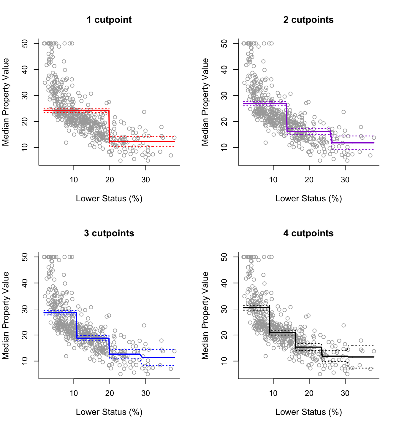

Note that we do not necessarily need to rely on the automatic selections of cutpoints used by cut(). We can define the intervals if we want to. For instance, if we want cutpoints at 10, 20 and 30 we can do the following

breaks4 = c(min(x), 10, 20, 30, max(x))
table(cut(x, breaks = breaks4))

## 
## (1.73,10]   (10,20]   (20,30]   (30,38] 
##       218       213        62        12

Note that when defining the sequence of breaks, we included min(x) and max(x) at the start and end in order to ensure the intervals covered the entire range of x.

Then our model would be:

step.new4 = lm(y ~ cut(x, breaks = breaks4))
summary(step.new4)

## 
## Call:
## lm(formula = y ~ cut(x, breaks = breaks4))
## 
## Residuals:
##      Min       1Q   Median       3Q      Max 
## -17.4803  -4.6239  -0.4239   2.8968  20.6197 
## 
## Coefficients:
##                                 Estimate Std. Error t value            Pr(>|t|)
## (Intercept)                      29.3803     0.4415  66.540 <0.0000000000000002
## cut(x, breaks = breaks4)(10,20] -10.4563     0.6281 -16.648 <0.0000000000000002
## cut(x, breaks = breaks4)(20,30] -16.6770     0.9383 -17.773 <0.0000000000000002
## cut(x, breaks = breaks4)(30,38] -18.6886     1.9331  -9.668 <0.0000000000000002
##                                    
## (Intercept)                     ***
## cut(x, breaks = breaks4)(10,20] ***
## cut(x, breaks = breaks4)(20,30] ***
## cut(x, breaks = breaks4)(30,38] ***
## ---
## Signif. codes:  0 '***' 0.001 '**' 0.01 '*' 0.05 '.' 0.1 ' ' 1
## 
## Residual standard error: 6.519 on 501 degrees of freedom
##   (1 observation deleted due to missingness)
## Multiple R-squared:  0.4925, Adjusted R-squared:  0.4895 
## F-statistic: 162.1 on 3 and 501 DF,  p-value: < 0.00000000000000022

Although somewhat trivial, we can make predictions at new data points using the constructed linear model as usual.

newx <- c(10.56, 5.89)
preds = predict(step.new4, newdata = list(x = newx), se = TRUE)
preds

## $fit
##        1        2 
## 18.92394 29.38028 
## 
## $se.fit
##         1         2 
## 0.4466955 0.4415432 
## 
## $df
## [1] 501
## 
## $residual.scale
## [1] 6.519307