Practical Class Sheets 3
In this practical class, we will apply ridge and lasso regression for multiple linear regression and explore principal component analysis.
To start, create a new R script by clicking on the corresponding menu button (in the top left); and save it somewhere in your computer. You can now write all your code into this file, and then execute it in R using the menu button Run or by simple pressing ctrl \(+\) enter.
In this practical class we will investigate the dataset seatpos from the library faraway.
Initial Data Analysis
Exercise 3.1
This exercise focuses on generally improving your data analytical skills which you have been practicing since the first practical class.
Load library
farawayand check the help file for datasetseatpos.Looking at the help file, which variable might the researchers at the HuMoSim laboratory consider to be a good response variable?
Looking at the help document only for the moment (that is, without performing any analysis on the dataset), are there any predictor variables that we think may be likely to be highly correlated?
What is the dimension of the dataset? Check whether there is any missing data.
Use exploratory data analysis commands and plots to investigate the correlation of
hipcenterwith the other (possible predictor) variables. With which predictor variables ishipcentermost correlated? Are those predictor variables correlated with each other? Does this exploratory analysis support your initial thoughts from part (c)? What do your findings here suggest about the fixed location referred to in the help document for description ofhipcenter(is it in front or behind the driver)?
Click for solution
## SOLUTION

# (a)
library(faraway)
?seatpos

# (b)
# hipcenter would be a good response variable, as it is the only variable
# in the dataset that considers the location of a person within the car.
# This can be used as a proxy for where different drivers will position the
# seat, which is the quantity of interest for car designers.


# (c)
# Many of the predictors could be highly correlated.
# Examples include:
# - height and weight (a whole analysis could be done on this
# pairing),
# - lower leg length and thigh length - I would suspect people with
# longer lower legs also have longer thighs, but maybe I'm wrong.
# - Ht and HtShoes - these two variables measure height bare foot and in
# shoes - given that people's heights are in general not going to increase
# much by putting on a pair of shoes (and possibly by roughly a similar
# amount for each person), these variables are likely to be (very) highly
# correlated.  I would question including both of these variables
# in an analysis, although our computational analyses will confirm whether
# this is the case.
#
# Perhaps Age is unlikely to be too highly correlated with any of the other
# variables.
# Note that the aim of this question is to get you to think about the
# dataset before we go headlong into applying computational methods, since
# this is what a statistician/data scientist/machine learner should do!

# (d)
dim( seatpos ) # 38 samples, 9 variables.
## [1] 38 9sum(is.na(seatpos)) # no missing data.## [1] 0# (e)
# We can calculate the correlation of `hipcenter` to the other variables.
# Note that the response is the ninth variable in this dataset.
cor(seatpos[,9], seatpos[,-9]) ## Age Weight HtShoes Ht Seated Arm Thigh
## [1,] 0.2051722 -0.640333 -0.7965964 -0.7989274 -0.7312537 -0.585095 -0.5912015
## Leg
## [1,] -0.7871685# From this we see that `hipcenter` has a reasonable negative correlation
# with most of the predictors, apart from age.
# We display the correlation matrix across the eight predictors as follows.
cor( seatpos[,-9] )## Age Weight HtShoes Ht Seated Arm
## Age 1.00000000 0.08068523 -0.07929694 -0.09012812 -0.1702040 0.3595111
## Weight 0.08068523 1.00000000 0.82817733 0.82852568 0.7756271 0.6975524
## HtShoes -0.07929694 0.82817733 1.00000000 0.99814750 0.9296751 0.7519530
## Ht -0.09012812 0.82852568 0.99814750 1.00000000 0.9282281 0.7521416
## Seated -0.17020403 0.77562705 0.92967507 0.92822805 1.0000000 0.6251964
## Arm 0.35951115 0.69755240 0.75195305 0.75214156 0.6251964 1.0000000
## Thigh 0.09128584 0.57261442 0.72486225 0.73496041 0.6070907 0.6710985
## Leg -0.04233121 0.78425706 0.90843341 0.90975238 0.8119143 0.7538140
## Thigh Leg
## Age 0.09128584 -0.04233121
## Weight 0.57261442 0.78425706
## HtShoes 0.72486225 0.90843341
## Ht 0.73496041 0.90975238
## Seated 0.60709067 0.81191429
## Arm 0.67109849 0.75381405
## Thigh 1.00000000 0.64954120
## Leg 0.64954120 1.00000000# Many of the predictors are reasonably highly correlated with each other,
# except for Age.
# As suspected the pairing with greatest correlation is Ht and HtShoes.
# We could obtain a pairs plot across the dataset.
pairs( seatpos, pch = 16, col = 2 )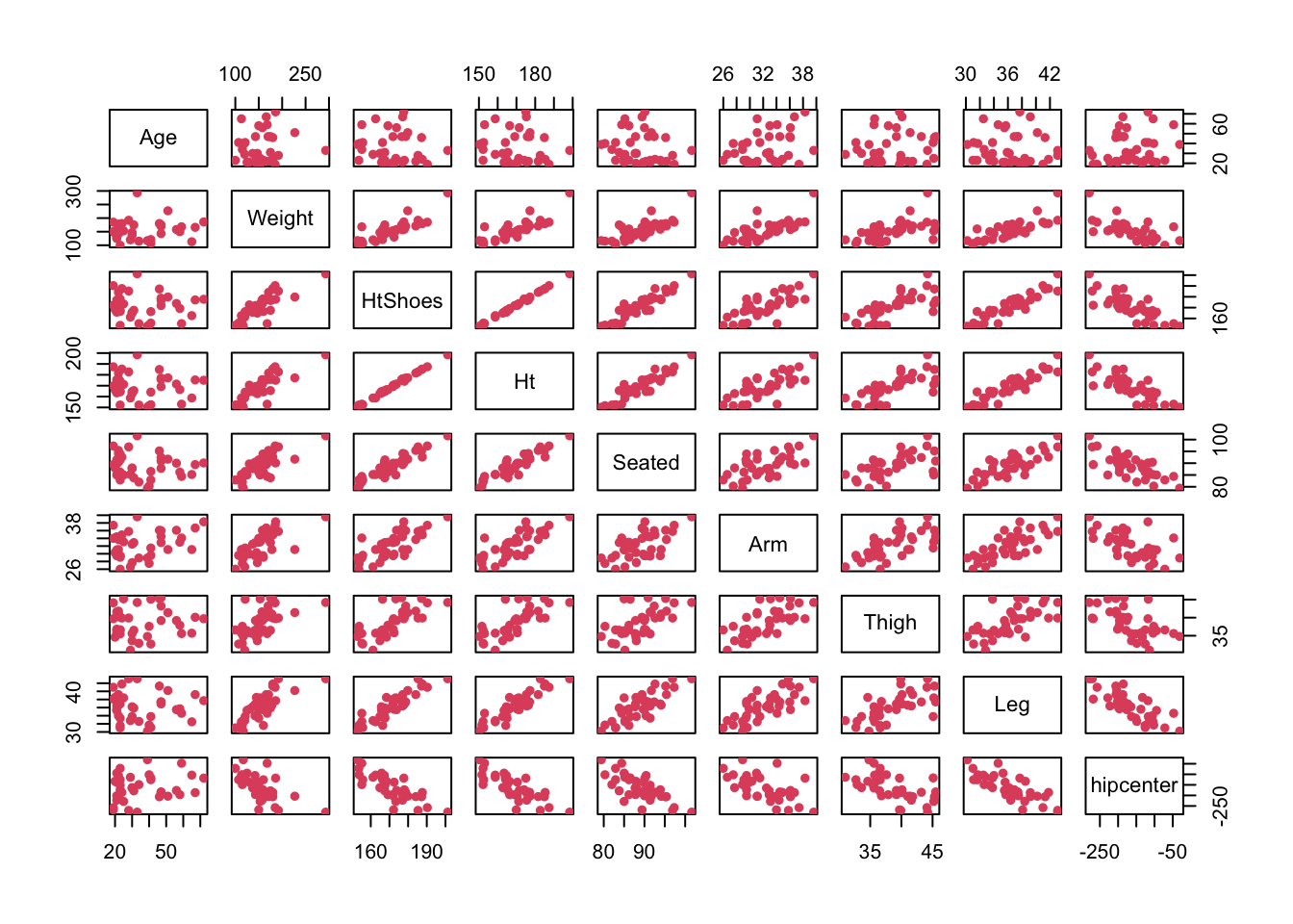
# These support the comments and correlations seen above.

# I would hazard a guess that the fixed location in the car is behind the
# driver, since the distance from it to the drivers hips gets smaller as
# the driver's various dimensions (in general) get larger.  Larger drivers
# are likely to move their seat back, so to make the distance shorter, the
# fixed position should be behind the driver.
# Note: these are my interpretations of the dataset, but again the purpose
# of this question is about getting you to think logically about the data
# you have been presented with.
# This can sometimes be harder than the computational side of things.
# In particular it may help to catch any coding errors (and potential
# illogical reasonings and conclusions) later!
Ridge Regression
Exercise 3.2
Define a vector
ycontaining all the values of the response variablehipcenter.Stack the predictors column-wise into a matrix, and define this matrix as
x.Load library
glmnet. Fit a model of all of the remaining variables forhipcenterusing ridge regression over a grid of 200 \(\lambda\) values. Hint: type?glmnetand look at argumentnlambda.Plot the regularisation paths of the ridge regresssion coefficients as a function of log \(\lambda\).
Click for solution
## SOLUTION

#(a)
y = seatpos$hipcenter

#(b)
x = model.matrix(hipcenter~., seatpos)[,-1]

#(c)
library("glmnet")
ridge = glmnet(x, y, alpha = 0, nlambda = 200)

#(d)
plot(ridge, xvar = 'lambda')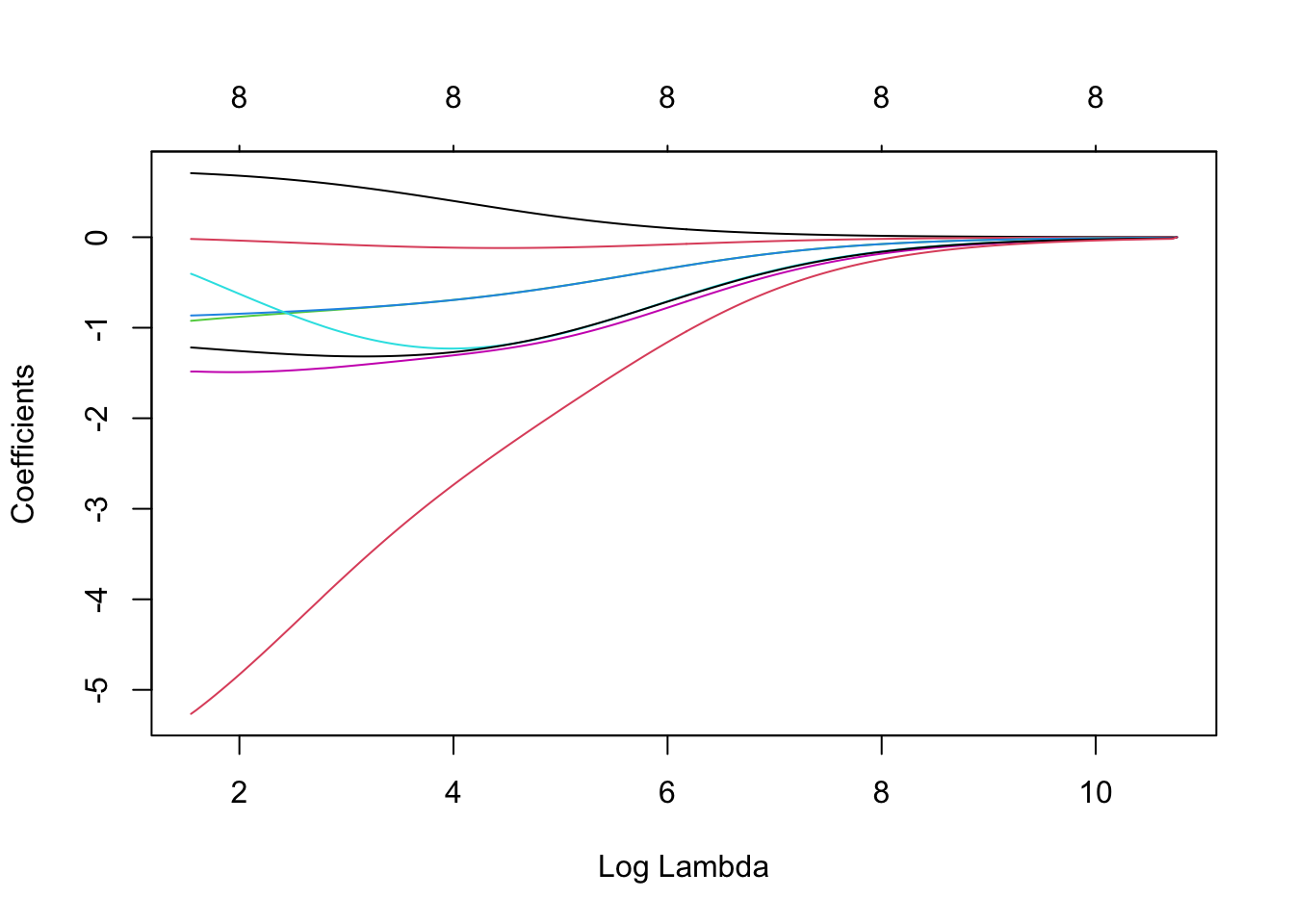
Lasso Regression
Exercise 3.3
Fit a model of all of the remaining variables for hipcenter using lasso regression. Plot regularisation paths against log \(\lambda\) and \(\ell_1\) norm values. Investigate which variables are included under various values of \(\lambda\). Do you notice anything interesting about the trends for the predictors Ht and HtShoes? Do the findings here support exploratory analysis of Exercise 3.1?
Click for solution
## SOLUTION


lasso = glmnet(x, y)
par(mfrow = c(1,2))
plot(lasso, xvar = 'lambda')
plot(lasso)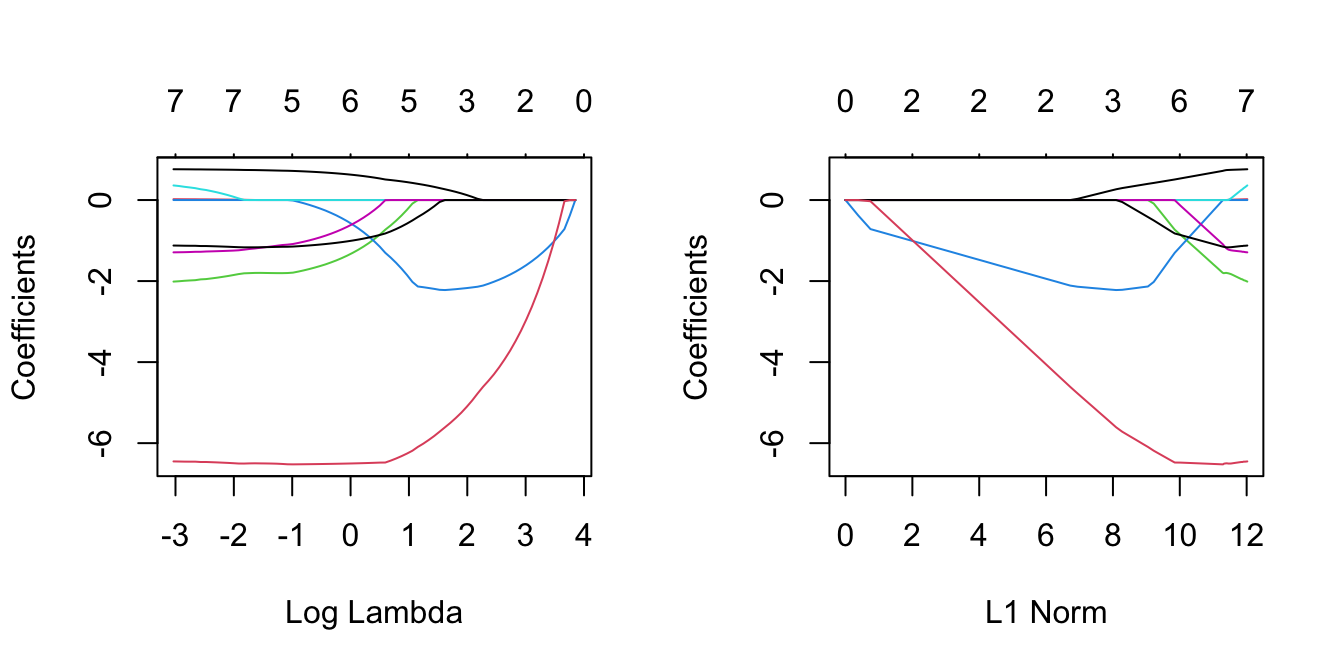
# We can see which values of lambda were in the grid.
lasso$lambda
## [1] 47.02272566 42.84535631 39.03909294 35.57096752 32.41094081 29.53164215
## [7] 26.90813246 24.51768813 22.33960429 20.35501542 18.54673195 16.89909140
## [13] 15.39782269 14.02992256 12.78354291 11.64788819 10.61312191 9.67028141
## [19] 8.81120026 8.02843751 7.31521325 6.66534987 6.07321856 5.53369056
## [25] 5.04209274 4.59416712 4.18603397 3.81415825 3.47531895 3.16658119
## [31] 2.88527084 2.62895133 2.39540254 2.18260158 1.98870527 1.81203418
## [37] 1.65105806 1.50438261 1.37073740 1.24896487 1.13801027 1.03691258
## [43] 0.94479612 0.86086304 0.78438634 0.71470362 0.65121132 0.59335950
## [49] 0.54064708 0.49261748 0.44885470 0.40897969 0.37264706 0.33954212
## [55] 0.30937814 0.28189383 0.25685116 0.23403321 0.21324235 0.19429849
## [61] 0.17703754 0.16131002 0.14697968 0.13392241 0.12202511 0.11118474
## [67] 0.10130739 0.09230752 0.08410718 0.07663533 0.06982726 0.06362399
## [73] 0.05797181 0.05282176 0.04812922# We can see which variables were included under each of those.
lasso$beta## 8 x 75 sparse Matrix of class "dgCMatrix"## [[ suppressing 75 column names 's0', 's1', 's2' ... ]]##
## Age . . . . . . .
## Weight . . . . . . .
## HtShoes . . . . . . .
## Ht . -0.3788888 -0.71690000 -0.8815363 -1.031066 -1.168389 -1.292464
## Seated . . . . . . .
## Arm . . . . . . .
## Thigh . . . . . . .
## Leg . . -0.03001398 -0.5709448 -1.065255 -1.512438 -1.923026
##
## Age . . . . . . .
## Weight . . . . . . .
## HtShoes . . . . . . .
## Ht -1.406576 -1.509502 -1.604347 -1.689716 -1.768569 -1.839363 -1.904943
## Seated . . . . . . .
## Arm . . . . . . .
## Thigh . . . . . . .
## Leg -2.293971 -2.635099 -2.942743 -3.226199 -3.481281 -3.716848 -3.928280
##
## Age . . . . 0.03026313 0.07914329
## Weight . . . . . .
## HtShoes . . . . . .
## Ht -1.963641 -2.017036 -2.066746 -2.111083 -2.13956040 -2.15657249
## Seated . . . . . .
## Arm . . . . . .
## Thigh . . . . . .
## Leg -4.124080 -4.302752 -4.462389 -4.610703 -4.77565830 -4.94857151
##
## Age 0.123651 0.164252 0.2011991 0.2349099 0.2656318 0.29557296
## Weight . . . . . .
## HtShoes . . . . . .
## Ht -2.172738 -2.186422 -2.1999306 -2.2112247 -2.2213847 -2.21537008
## Seated . . . . . .
## Arm . . . . . .
## Thigh . . . . . -0.04904616
## Leg -5.104146 -5.249008 -5.3779072 -5.4983751 -5.6085302 -5.71786751
##
## Age 0.3254539 0.3526374 0.3774918 0.4000568 0.42215302 0.4425705
## Weight . . . . . .
## HtShoes . . . . -0.08747275 -0.2410930
## Ht -2.1919535 -2.1710512 -2.1509204 -2.1336034 -2.02086133 -1.8495163
## Seated . . . . . .
## Arm . . . . . .
## Thigh -0.1550600 -0.2512560 -0.3396447 -0.4194801 -0.50353183 -0.5808560
## Leg -5.8252121 -5.9220281 -6.0129224 -6.0932133 -6.18702261 -6.2568841
##
## Age 0.4611742 0.4781344 0.4935876 0.507660431 0.5325412 0.5538978
## Weight . . . . . .
## HtShoes -0.3810765 -0.5094711 -0.6264423 -0.732315652 -0.8541160 -0.9612630
## Ht -1.6933835 -1.5502583 -1.4198654 -1.301776165 -1.1523513 -1.0218632
## Seated . . . . . .
## Arm . . . -0.003724438 -0.1356874 -0.2445963
## Thigh -0.6513109 -0.7155662 -0.7741120 -0.825232452 -0.8617522 -0.8945363
## Leg -6.3205372 -6.3785468 -6.4314027 -6.478380251 -6.4798559 -6.4847698
##
## Age 0.5733715 0.5910974 0.6072458 0.6219709 0.6353911 0.6476155
## Weight . . . . . .
## HtShoes -1.0599721 -1.1485746 -1.2290941 -1.3032866 -1.3710911 -1.4325446
## Ht -0.9018626 -0.7938899 -0.6957256 -0.6054368 -0.5229599 -0.4481416
## Seated . . . . . .
## Arm -0.3438619 -0.4342699 -0.5166409 -0.5917202 -0.6601388 -0.7224752
## Thigh -0.9244800 -0.9516743 -0.9764387 -0.9990584 -1.0196829 -1.0384553
## Leg -6.4892510 -6.4933288 -6.4970433 -6.5004312 -6.5035202 -6.5063374
##
## Age 0.6587657 0.6689108 0.6781749 0.6865932 0.6942714 0.7012737
## Weight . . . . . .
## HtShoes -1.4893806 -1.5398858 -1.5875253 -1.6288279 -1.6673273 -1.7029099
## Ht -0.3791066 -0.3175022 -0.2597176 -0.2091840 -0.1622689 -0.1190003
## Seated . . . . . .
## Arm -0.7793014 -0.8310560 -0.8782503 -0.9212114 -0.9603579 -0.9960311
## Thigh -1.0556179 -1.0711783 -1.0854622 -1.0983601 -1.1101614 -1.1209538
## Leg -6.5089124 -6.5112740 -6.5134288 -6.5154515 -6.5172794 -6.5189702
##
## Age 0.70765527 0.71346592 0.7187507 0.7228005 0.7250685 0.7283275
## Weight . . . . . .
## HtShoes -1.73553063 -1.76517488 -1.7918480 -1.8012793 -1.8042393 -1.8036976
## Ht -0.07936592 -0.04332879 -0.0108381 . . .
## Seated . . . . . .
## Arm -1.02852223 -1.05809285 -1.0849764 -1.1006536 -1.1107097 -1.1284351
## Thigh -1.13080691 -1.13978543 -1.1479486 -1.1525898 -1.1535925 -1.1565048
## Leg -6.52053931 -6.52200063 -6.5233662 -6.5216161 -6.5131065 -6.5068898
##
## Age 0.731506 0.734511 0.737307 0.739810222 0.741186412 0.742529970
## Weight . . . 0.001075362 0.003693442 0.006652873
## HtShoes -1.802075 -1.800008 -1.797816 -1.798603166 -1.803557433 -1.808553585
## Ht . . . . . .
## Seated . . . . . 0.002378954
## Arm -1.145882 -1.162368 -1.177701 -1.194759877 -1.207604764 -1.224531973
## Thigh -1.159510 -1.162575 -1.165548 -1.166929365 -1.167273424 -1.167232842
## Leg -6.503318 -6.501111 -6.499640 -6.497567833 -6.499442317 -6.503591032
##
## Age 0.745354326 0.74742495 0.7490595 0.75051743 0.75188196 0.75309161
## Weight 0.008513292 0.01013531 0.0117728 0.01326849 0.01463865 0.01587222
## HtShoes -1.827269779 -1.85186185 -1.8757287 -1.89667200 -1.91673747 -1.93407617
## Ht . . . . . .
## Seated 0.040515474 0.08294766 0.1225952 0.15754489 0.19096305 0.21992109
## Arm -1.239936898 -1.24773622 -1.2530833 -1.25803785 -1.26232015 -1.26641490
## Thigh -1.163875042 -1.15825820 -1.1526247 -1.14780561 -1.14306697 -1.13909162
## Leg -6.502812684 -6.49475353 -6.4872853 -6.48122990 -6.47512351 -6.47010118
##
## Age 0.75422793 0.75592912 0.75628200 0.75774078 0.75870481 0.75951416
## Weight 0.01700937 0.01736582 0.01888635 0.01919551 0.01980897 0.02057163
## HtShoes -1.95075883 -1.95798264 -1.97774056 -1.98463485 -1.99295752 -2.00426952
## Ht . . . . . .
## Seated 0.24771599 0.26649454 0.29335360 0.31078418 0.32692789 0.34634309
## Arm -1.26997742 -1.27709493 -1.27745387 -1.28286904 -1.28666067 -1.28881721
## Thigh -1.13514900 -1.13506802 -1.12899125 -1.12874195 -1.12739244 -1.12473708
## Leg -6.46501672 -6.46519803 -6.45672861 -6.45697888 -6.45593029 -6.45313255
##
## Age 0.76009998
## Weight 0.02118573
## HtShoes -2.01275176
## Ht .
## Seated 0.36049535
## Arm -1.29085662
## Thigh -1.12283674
## Leg -6.45077390# In particular, high values of lambda leads to inclusion of Ht only.
# Other variables start to come in; leg, followed by Age,
# followed by Thigh, as lambda gets smaller.
# It is interesting that Age comes in third, despite having a reasonably
# small correlation with the response.
# However, this may be as expected, since the other variables also have
# high correlations with each other (collinearity), whereas Age may
# contain alternative predictive information.
# Interestingly, HtShoes enters only for small enough values of lambda, at
# which point its coefficients increase whilst the Ht coefficients
# decrease, eventually to zero.
# This is to do with the ridiculously high correlation between Ht
# and HtShoes (spotted in Exercise 3.1) - even for really low values of lambda,
# we don't need both of these variables.Principal Component Analysis
Exercise 3.4
Conduct Principal Component Analysis to all the predictors
xas in Exercise 3.2 with all variables being scaled to have unit variance.Report the variance of each of the principal component and the eigenvectors that corresponding to the first principal component.
Draw a scree plot. How many components would you need in order to capture at least
\(95\%\) of the total variance of the data cloud?Compress the data using the number of principal components as in (c), then reconstruct the data and compare the reconstruct data with the original data by looking at
Ageandweight.
Click for solution
## SOLUTION

#(a)
s <- apply(x, 2, sd)       # calculates the column standard deviations
x.s  <- sweep(x, 2, s, "/")  # divides all columns by their standard deviations
seatpos.pr <- prcomp(x.s)

#(b)
seatpos.pr
## Standard deviations (1, .., p=8):
## [1] 2.38184501 1.11210881 0.68098711 0.49087508 0.44070349 0.37306059 0.22437586
## [8] 0.03985271
##
## Rotation (n x k) = (8 x 8):
## PC1 PC2 PC3 PC4 PC5 PC6
## Age -0.007219379 0.8763467 0.16383976 -0.16522774 -0.3349932 -0.25464449
## Weight -0.366979122 0.0448877 0.42981137 -0.60025209 0.5537489 0.09798202
## HtShoes -0.411460536 -0.1055831 0.03375209 0.02577245 -0.2204816 -0.05101900
## Ht -0.412057421 -0.1119799 0.01116858 0.02294603 -0.1887759 -0.04369735
## Seated -0.381270226 -0.2178995 0.17138740 -0.15033847 -0.6171009 0.23019712
## Arm -0.348771387 0.3742641 -0.01670980 0.55358297 0.2380225 0.60781701
## Thigh -0.327523319 0.1251793 -0.86246173 -0.31151283 0.1038969 -0.06344739
## Leg -0.389747512 -0.0555930 0.11688322 0.43024468 0.2205229 -0.70326773
## PC7 PC8
## Age 0.02269849 -0.015528966
## Weight -0.04435483 0.008082356
## HtShoes 0.53650776 0.691876699
## Ht 0.50884054 -0.721493879
## Seated -0.56689080 -0.002844309
## Arm -0.07347462 0.007539785
## Thigh -0.14492761 0.018814564
## Leg -0.32092126 0.005274142seatpos.pr$rotation[,1]## Age Weight HtShoes Ht Seated Arm
## -0.007219379 -0.366979122 -0.411460536 -0.412057421 -0.381270226 -0.348771387
## Thigh Leg
## -0.327523319 -0.389747512#(c)
plot(seatpos.pr)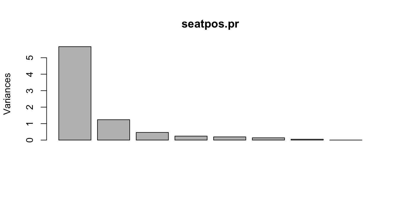
summary(seatpos.pr)## Importance of components:
## PC1 PC2 PC3 PC4 PC5 PC6 PC7
## Standard deviation 2.3818 1.1121 0.68099 0.49088 0.44070 0.3731 0.22438
## Proportion of Variance 0.7091 0.1546 0.05797 0.03012 0.02428 0.0174 0.00629
## Cumulative Proportion 0.7091 0.8638 0.92171 0.95183 0.97611 0.9935 0.99980
## PC8
## Standard deviation 0.03985
## Proportion of Variance 0.00020
## Cumulative Proportion 1.00000# 4 components are needed to capture at least
# 95% of the total variance of the data cloud
#(d)
T <- t(seatpos.pr$x[,c(1,2,3,4)]) #compressed using 4 PCs
ms <- colMeans(x.s)
R <- t(ms + seatpos.pr$rot[,c(1,2,3,4)]%*% T) #reconstruction
plot(rbind(x.s[,1:2], R[,1:2]), col=c(rep(1,38),rep(3,38))) 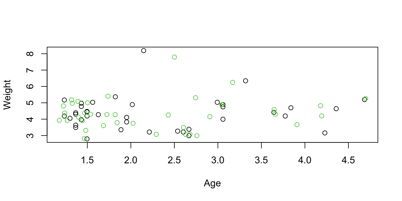
Principal Component Regression
Exercise 3.5
Load library
pls(required for PCR). Use the commandpcrto fit a principal component regression model tohipcenterbased on the remaining variables. Select the number of principal components using cross-validation. Remember to standardise the variables. How many principal components are recommended, according to the cross-validation error?Appropriately plot the mean squared validation error.
Use the command
coef()to find corresponding coefficient estimates in terms of the original \(\hat{\beta}\)’s. How do these estimates coincide with the exploratory analysis of Exercise 3.1?
Click for solution
## SOLUTION

#(a)
library("pls")
pcr.fit=pcr(hipcenter~., data=seatpos, scale = TRUE, validation = "CV" )
summary(pcr.fit)
## Data: X dimension: 38 8
## Y dimension: 38 1
## Fit method: svdpc
## Number of components considered: 8
##
## VALIDATION: RMSEP
## Cross-validated using 10 random segments.
## (Intercept) 1 comps 2 comps 3 comps 4 comps 5 comps 6 comps
## CV 60.45 37.89 36.83 38.04 37.68 38.05 39.64
## adjCV 60.45 37.80 36.69 37.84 37.42 37.81 39.28
## 7 comps 8 comps
## CV 43.57 43.93
## adjCV 42.96 43.30
##
## TRAINING: % variance explained
## 1 comps 2 comps 3 comps 4 comps 5 comps 6 comps 7 comps
## X 70.91 86.37 92.17 95.18 97.61 99.35 99.98
## hipcenter 61.89 66.34 66.48 67.82 68.02 68.58 68.63
## 8 comps
## X 100.00
## hipcenter 68.66# The summary suggests use of 2 principal components.
# Notice this is different from the number in Exercise 3.4c
#(b)
validationplot( pcr.fit, val.type = 'MSEP' )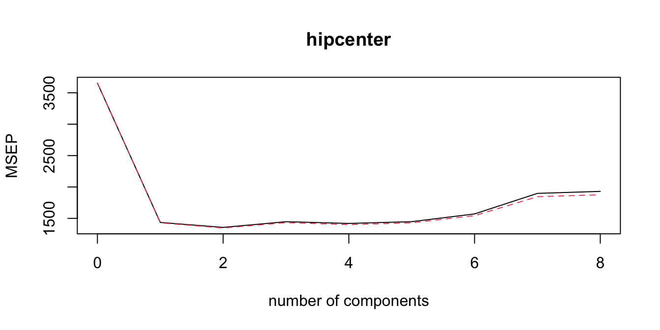
#(c)
coef(pcr.fit, ncomp = 2)
## , , 2 comps
##
## hipcenter
## Age 9.779064
## Weight -6.721580
## HtShoes -9.301406
## Ht -9.385585
## Seated -9.978190
## Arm -2.633940
## Thigh -5.035274
## Leg -8.307696# Since Age had a positive correlation with hipcenter, the coefficient
# is positive. For the remaining variables the correlation was negative,
# so the coefficients are negative.
# Notice how the size of the coefficients is relatively similar across
# all predictor variables.
# This is to do with how Principal Component Analysis works.Predictive Performance of Methods
Exercise 3.6
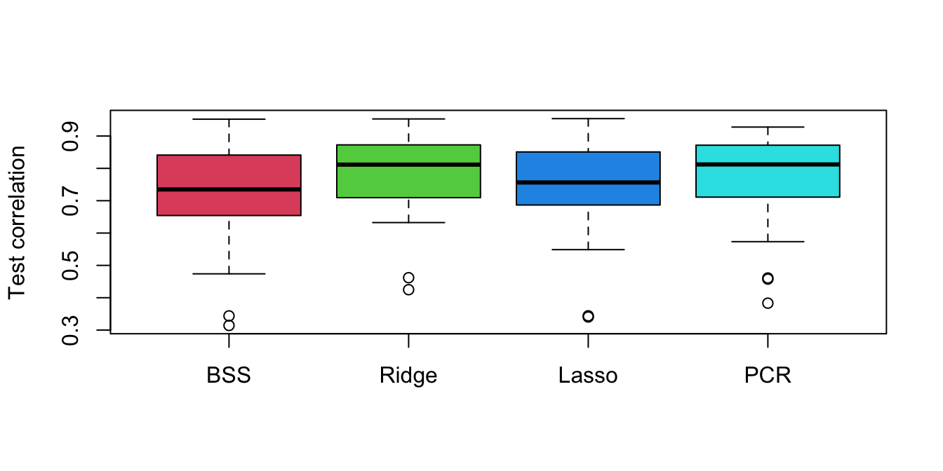
Use 50 repetitions of data-splitting with 28 samples for training (10 for testing) to compare the predictive performance (e.g. Correlation and MSE) of the following models of the remaining predictors for hipcenter:
- Best subset selection with \(C_p\)
- Ridge with min-CV \(\lambda\) (5 folds)
- Lasso with min-CV \(\lambda\) (5 folds)
- PCR with min-CV number of principal components.
Click for solution
# Load R libraries.
library(leaps)

# Predict function for regsubsets
predict.regsubsets = function(object, newdata, id, ...){
  form = as.formula(object$call[[2]])
  mat = model.matrix(form, newdata)
  coefi = coef(object, id = id)
  xvars = names(coefi)
  mat[, xvars]%*%coefi
}

repetitions = 50
cor.bss = c()
cor.ridge = c()
cor.lasso = c()
cor.pcr = c()

set.seed(1)
for(i in 1:repetitions){
  # Step (i) data splitting
  training.obs = sample(1:38,  28)
  y.train = seatpos$hipcenter[training.obs]
  x.train = model.matrix(hipcenter~., seatpos[training.obs, ])[,-1]
  y.test = seatpos$hipcenter[-training.obs]
  x.test = model.matrix(hipcenter~., seatpos[-training.obs, ])[,-1]

  # Step (ii) training phase
  bss.train = regsubsets(hipcenter~., data=seatpos[training.obs,], nvmax=8)
  min.cp = which.min(summary(bss.train)$cp)
  ridge.train = cv.glmnet(x.train, y.train, alpha = 0, nfolds = 5)
  lasso.train = cv.glmnet(x.train, y.train, nfold = 5)
  pcr.train = pcr(hipcenter~., data =seatpos[training.obs,],
                  scale = TRUE, validation="CV")
  min.pcr = which.min(MSEP(pcr.train)$val[1,1, ] ) - 1

  # Step (iii) generating predictions
  predict.bss = predict.regsubsets(bss.train, seatpos[-training.obs, ], min.cp)
  predict.ridge = predict(ridge.train, x.test, s = 'lambda.min')
  predict.lasso = predict(lasso.train, x.test, s = 'lambda.min')
  predict.pcr = predict(pcr.train,seatpos[-training.obs, ], ncomp = min.pcr )

  # Step (iv) evaluating predictive performance
  cor.bss[i] = cor(y.test, predict.bss)
  cor.ridge[i] = cor(y.test, predict.ridge)
  cor.lasso[i] = cor(y.test, predict.lasso)
  cor.pcr[i] = cor(y.test, predict.pcr)
}

# Plot the resulting correlations as boxplots.
boxplot(cor.bss, cor.ridge, cor.lasso, cor.pcr,
        names = c('BSS','Ridge', 'Lasso', 'PCR'),
        ylab = 'Test correlation', col = 2:5)