Chapter 3 Linear Regression
3.1 Simple Linear Regression: Introduction
Motivation: Predicting the Price of a Used Car

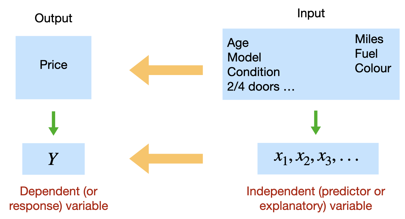
The table below displays data on Age (in years) and Price (in hundreds of dollars) for a sample of cars of a particular make and model. Weiss (2012)
| Price (\(y\)) | Age (\(x\)) |
|---|---|
| 85 | 5 |
| 103 | 4 |
| 70 | 6 |
| 82 | 5 |
| 89 | 5 |
| 98 | 5 |
| 66 | 6 |
| 95 | 6 |
| 169 | 2 |
| 70 | 7 |
| 48 | 7 |
Enter the data in R.
Price<-c(85, 103,  70,  82,  89,  98,  66,  95, 169,  70,  48)
Age<- c(5, 4, 6, 5, 5, 5, 6, 6, 2, 7, 7)
carSales<-data.frame(Price,Age)
str(carSales)
## 'data.frame': 11 obs. of 2 variables:
## $ Price: num 85 103 70 82 89 98 66 95 169 70 ...
## $ Age : num 5 4 6 5 5 5 6 6 2 7 ...cor(Age, Price, method = "pearson")## [1] -0.9237821Scatterplot: Age vs. Price
library(ggplot2)
ggplot(carSales, aes(x=Age, y=Price)) + geom_point()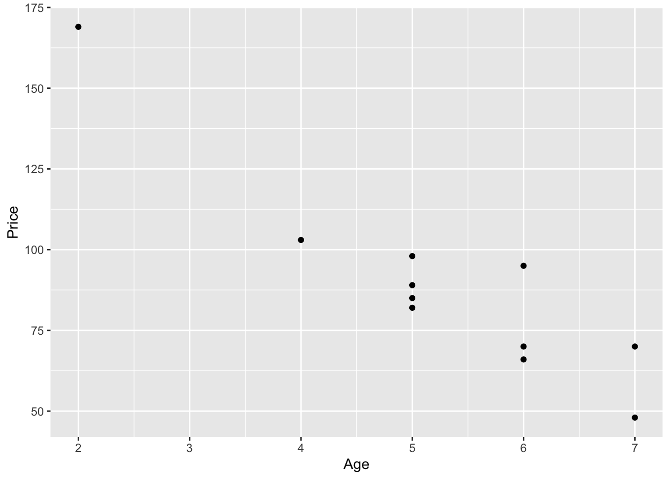
ggplot(carSales, aes(x=Age, y=Price)) +
  geom_point()+
  geom_smooth(method=lm, formula= y~x, se=FALSE)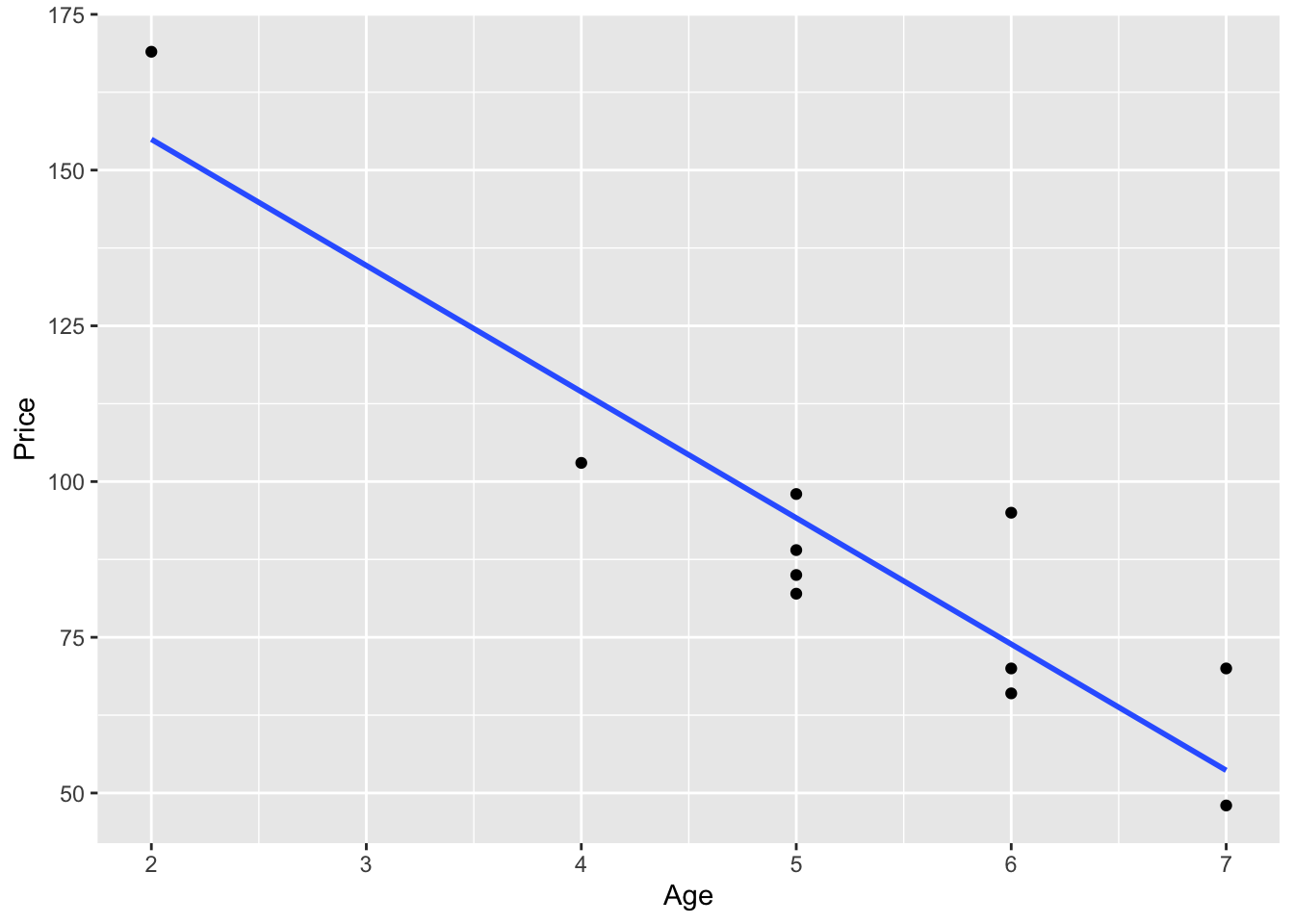
Obviously, we see a linear relationship between Age and Price.
Simple linear regression Model
Simple linear regression (population) \[Y=\beta_0+\beta_1 x+\epsilon\] In our example: \[Price=\beta_0+\beta_1 Age+\epsilon\]
Simple linear regression (sample) \[\hat{y}=b_0+b_1 x\] where the coefficient \(\beta_0\) (and its estimate \(b_0\) or \(\hat{\beta}_0\) ) refers to the \(y\)-intercept or simply the intercept or the constant of the regression line, and the coefficient \(\beta_1\) (and its estimate (and its estimate \(b_1\) or \(\hat{\beta}_1\) ) refers to the slope of the regression line.
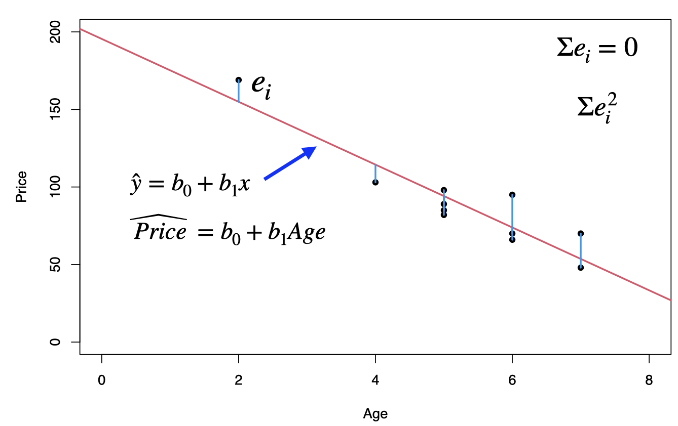
The Least Squares criterion
Recall that one of the four pillars we need for successful machine learning is performance metric. In order to estimate the simple linear regression model parameters (here coefficients \(\beta_0\) and \(\beta_1\)), we need to find the right performance metric. Here comes the least squares.
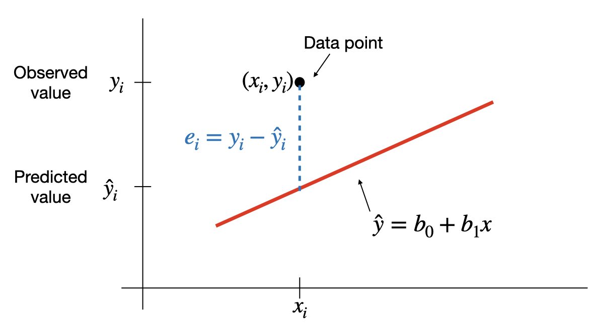
The least squares criterion is that the line that best fits a set of data points is the one having the smallest possible sum of squared errors. The `errors’ are the vertical distances of the data points to the line.
The regression line is the line that fits a set of data points according to the least squares criterion.
The regression equation is the equation of the regression line.
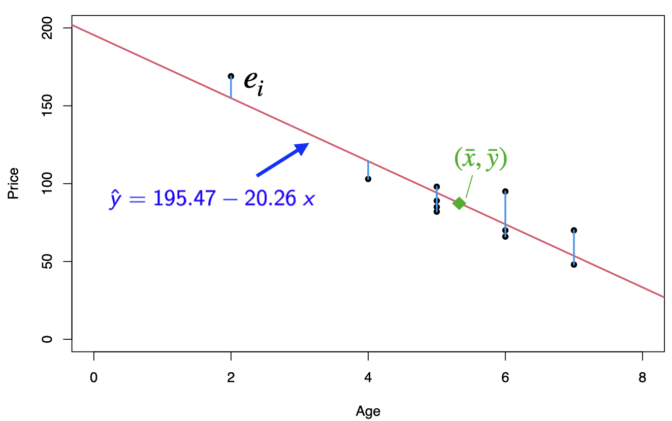
The regression equation for a set of \(n\) data points is \(\hat{y}=b_0+b_1\;x\), where \[b_1=\frac{S_{xy}}{S_{xx}}=\frac{\sum (x_i-\bar{x})(y_i-\bar{y})}{\sum (x_i-\bar{x})^2} \;\;\text{and}\;\; b_0=\bar{y}-b_1\; \bar{x}\]
\(y\) is the dependent variable (or response variable) and \(x\) is the independent variable (predictor variable or explanatory variable).
\(b_0\) is called the y-intercept and \(b_1\) is called the slope.
SSE and the standard error
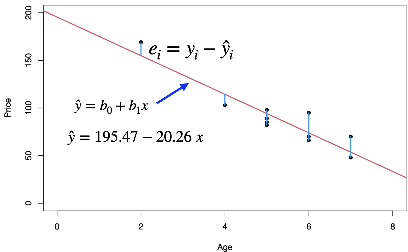
This least square regression line minimizes the error sum of squares \[SSE=\sum e^2_i =\sum (y_i-\hat{y}_i)^2\] The standard error of the estimate, \(s_e=\sqrt{SSE/(n-2)}\), indicates how much, on average, the observed values of the response variable differ from the predicted values of the response variable.
Prediction
# simple linear regression
reg<-lm(Price~Age)
print(reg)
##
## Call:
## lm(formula = Price ~ Age)
##
## Coefficients:
## (Intercept) Age
## 195.47 -20.26To predict the price of a 4-year-old car (\(x=4\)): \[\hat{y}=195.47-20.26(4)=114.43\]
 Note the prediction \(\hat{y}\) has not accounted for any uncertainty yet.
3.2 Simple Regression: Coefficient of Determination
Used cars example
The table below displays data on Age (in years) and Price (in hundreds of dollars) for a sample of cars of a particular make and model. Weiss (2012)
| Price (\(y\)) | Age (\(x\)) |
|---|---|
| 85 | 5 |
| 103 | 4 |
| 70 | 6 |
| 82 | 5 |
| 89 | 5 |
| 98 | 5 |
| 66 | 6 |
| 95 | 6 |
| 169 | 2 |
| 70 | 7 |
| 48 | 7 |
For our example, age is the predictor variable and price is the response variable.
The regression equation is \(\hat{y}=195.47-20.26\;x\), where the slope \(b_1=-20.26\) and the intercept \(b_0=195.47\)
Prediction: for \(x = 4\), that is we would like to predict the price of a 4-year-old car, \[\hat{y}=195.47-20.26 {\color{blue}(4)}= 114.43 \;\;\text{or}\;\; \$ 11443\]
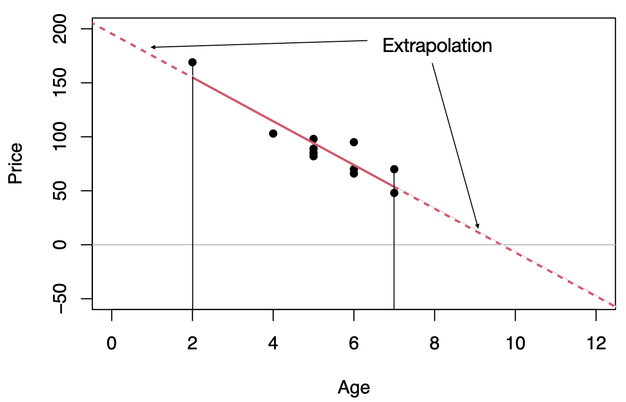
Extrapolation
Within the range of the observed values of the predictor variable, we can reasonably use the regression equation to make predictions for the response variable.
However, to do so outside the range, which is called Extrapolation, may not be reasonable because the linear relationship between the predictor and response variables may not hold here.
To predict the price of an 11-year old car, \(\hat{y}=195.47-20.26 (11)=-27.39\) or $ 2739, this result is unrealistic as no one is going to pay us $2739 to take away their 11-year old car.
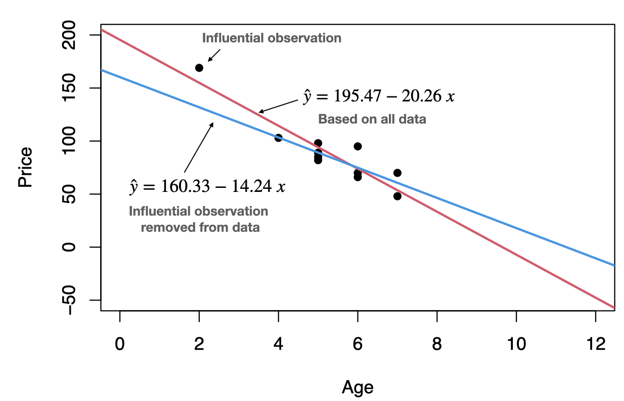
Outliers and influential observations
An outlier is an observation that lies outside the overall pattern of the data. In the context of regression, an outlier is a data point that lies far from the regression line, relative to the other data points.
An influential observation is a data point whose removal causes the regression equation (and line) to change considerably.
From the scatterplot, it seems that the data point (2,169) might be an influential observation. Removing that data point and recalculating the regression equation yields \(\hat{y}=160.33-14.24\;x\).
Coefficient of determination
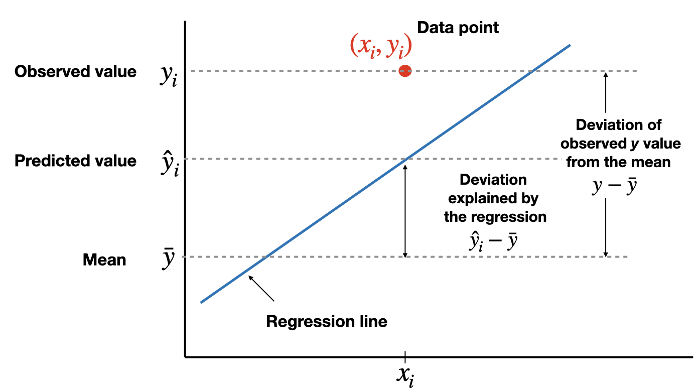
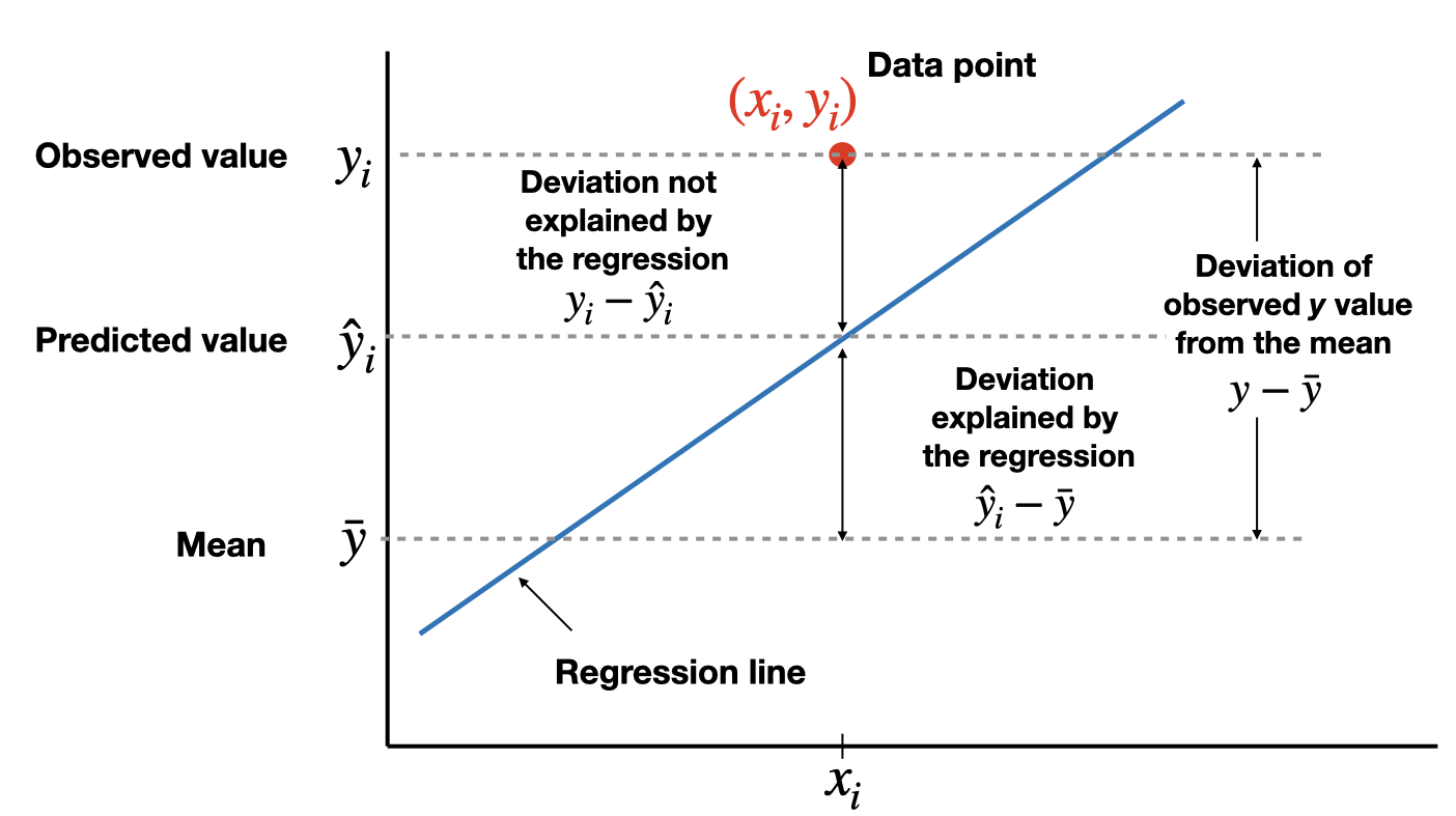
The total variation in the observed values of the response variable, \(SST=\sum(y_i-\bar{y})^2\), can be partitioned into two components:
- The variation in the observed values of the response variable explained by the regression: \(SSR=\sum(\hat{y}_i-\bar{y})^2\)
- The variation in the observed values of the response variable not explained by the regression: \(SSE=\sum(y_i-\hat{y}_i)^2\)
The coefficient of determination, \(R^2\) (or \(R\)-square), is the proportion of the variation in the observed values of the response variable explained by the regression, which is given by \[R^2=\frac{SSR}{SST}=\frac{SST-SSE}{SST}=1-\frac{SSE}{SST}\] where \(SST=SSR+SSE\). \(R^2\) is a descriptive measure of the utility of the regression equation for making prediction.
The coefficient of determination \(R^2\) always lies between 0 and 1. A value of \(R^2\) near 0 suggests that the regression equation is not very useful for making predictions, whereas a value of \(R^2\) near 1 suggests that the regression equation is quite “useful” for making predictions.
For a simple linear regression (one independent variable) ONLY, \(R^2\) is the square of Pearson correlation coefficient, \(r\).
\(\text{Adjusted}\;R^2\) is a modification of \(R^2\) which takes into account the number of independent variables, say \(k\). In a simple linear regression \(k=1\). Adjusted-\(R^2\) increases only when a significant related independent variable is added to the model. Adjusted-\(R^2\) has a crucial role in the process of model building. Adjusted-\(R^2\) is given by \[\text{Adjusted-}R^2=1-(1-R^2)\frac{n-1}{n-k-1}\]
Notation used in regression
| Quantity | Defining formula | Computing formula |
|---|---|---|
| \(S_{xx}\) | \(\sum (x_i-\bar{x})^2\) | \(\sum x^2_i - n \bar{x}^2\) |
| \(S_{xy}\) | \(\sum (x_i-\bar{x})(y_i-\bar{y})\) | \(\sum x_i y_i - n \bar{x}\bar{y}\) |
| \(S_{yy}\) | \(\sum (y_i-\bar{y})^2\) | \(\sum y^2_i - n \bar{y}^2\) |
where \(\bar{x}=\frac{\sum x_i}{n}\) and \(\bar{y}=\frac{\sum y_i}{n}\). And,
\[SST=S_{yy},\;\;\; SSR=\frac{S^2_{xy}}{S_{xx}},\;\;\; SSE=S_{yy}-\frac{S^2_{xy}}{S_{xx}} \] and \(SST=SSR+SSE\).
Proof \(R^2\) is the square of Pearson correlation coefficient
Suppose that we have \(n\) observations \((x_1,y_1)\),…,\((x_n,y_n)\) from a simple linear regression \[Y_i=\beta_0+\beta_1 x_i+\epsilon_i\] where \(i=1,...,n\). Let us denote \(\hat{y}_i=\hat{\beta}_0+\hat{\beta}_1 x_i\) for \(i=1,...,n\), where \(\hat{\beta}_0\) and \(\hat{\beta}_1\) are the least squares estimators of the parameters \(\beta_0\) and \(\beta_1\). The coefficient of the determination \(R^2\) is defined by \[R^2=\frac{\sum_{i=1}^{n}(\hat{y}_i-\bar{y})^2}{\sum_{i=1}^{n}({y}_i-\bar{y})^2}\] Using the facts that \[\hat{\beta}_1=\frac{\sum_{i=1}^{n} (x_i-\bar{x})(y_i-\bar{y})}{\sum_{i=1}^{n} (x_i-\bar{x})^2}\] and \(\hat{\beta}_0=\bar{y}-\hat{\beta}_1 \bar{x}\), we obtain
\[\begin{equation} \begin{split} \sum_{i=1}^{n}(\hat{y}_i-\bar{y})^2 & = \sum_{i=1}^{n}(\hat{\beta}_0+\hat{\beta}_1 x_i-\bar{y})^2\\ & =\sum_{i=1}^{n}(\bar{y}-\hat{\beta}_1 \bar{x}+\hat{\beta}_1 x_i-\bar{y})^2\\ & =\hat{\beta}_1^2 \sum_{i=1}^{n}(x_i-\bar{x})^2\\ & =\frac{[\sum_{i=1}^{n} (x_i-\bar{x})(y_i-\bar{y})]^2\sum_{i=1}^{n}(x_i-\bar{x})^2}{[\sum_{i=1}^{n} (x_i-\bar{x})^2]^2}\\ & =\frac{[\sum_{i=1}^{n} (x_i-\bar{x})(y_i-\bar{y})]^2}{\sum_{i=1}^{n} (x_i-\bar{x})^2} \end{split} \end{equation}\] Hence, \[\begin{equation} \begin{split} R^2 & = \frac{\sum_{i=1}^{n}(\hat{y}_i-\bar{y})^2}{\sum_{i=1}^{n}({y}_i-\bar{y})^2}\\ & =\frac{[\sum_{i=1}^{n} (x_i-\bar{x})(y_i-\bar{y})]^2}{\sum_{i=1}^{n} (x_i-\bar{x})^2\sum_{i=1}^{n}({y}_i-\bar{y})^2}\\ & =\left(\frac{\sum_{i=1}^{n} (x_i-\bar{x})(y_i-\bar{y})}{\sqrt{\sum_{i=1}^{n} (x_i-\bar{x})^2\sum_{i=1}^{n}({y}_i-\bar{y})^2}}\right)^2\\ & = r^2 \end{split} \end{equation}\]
This shows that the coefficient of determination of a simple linear regression is the square of the sample correlation coefficient of \((x_1,y_1)\),…,\((x_n,y_n)\).
3.3 Simple Linear Regression: Assumptions
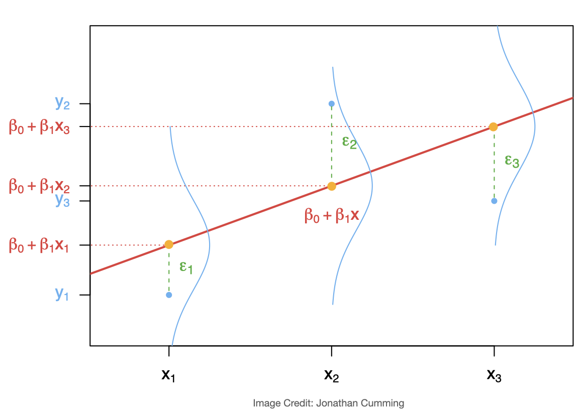
Recall that the simple linear regression model for \(Y\) on \(x\) is \[Y=\beta_0+\beta_1 x+\epsilon\] where
\(Y\) : the dependent or response variable
\(x\) : the independent or predictor variable, assumed known
\(\beta_0,\beta_1\) : the regression parameters, the intercept and slope of the regression line
\(\epsilon\) : the random regression error around the line.
and the regression equation for a set of \(n\) data points is \(\hat{y}=b_0+b_1\;x\), where \[b_1=\frac{S_{xy}}{S_{xx}}=\frac{\sum (x_i-\bar{x})(y_i-\bar{y})}{\sum (x_i-\bar{x})^2}\] and \[b_0=\bar{y}-b_1\; \bar{x}\] where \(b_0\) is called the y-intercept and \(b_1\) is called the slope.
The residual standard error \(s_e\) can be defined as
\[s_e=\sqrt{\frac{SSE}{n-2}}=\sqrt{\frac{\sum(y_i-\hat{y}_i)^2}{n-2}} \] \(s_e\) indicates how much, on average, the observed values of the response variable differ from the predicted values of the response variable. \(~\)
Simple Linear Regression Assumptions (SLR)
We have a collection of \(n\) pairs of observations \(\{(x_i,y_i)\}\), and the idea is to use them to estimate the unknown parameters \(\beta_0\) and \(\beta_1\). \[\epsilon_i=Y_i-(\beta_0+\beta_1\;x_i)\;,\;\;i=1,2,\ldots,n\]
We need to make the following key assumptions on the errors:
A. \(E(\epsilon_i)=0\) (errors have mean zero and do not depend on \(x\))
B. \(Var(\epsilon_i)=\sigma^2\) (errors have a constant variance, homoscedastic, and do not depend on \(x\))
C. \(\epsilon_1, \epsilon_2,\ldots \epsilon_n\) are independent.
D. \(\epsilon_i \mbox{ are all i.i.d. } N(0, \;\sigma^2)\), meaning that the errors are independent and identically distributed as Normal with mean zero and constant variance \(\sigma^2\).
The above assumptions, and conditioning on \(\beta_0\) and \(\beta_1\), imply:
Linearity: \(E(Y_i|X_i)=\beta_0+\beta_1\;x_i\)
Homogenity or homoscedasticity: \(Var(Y_i|X_i)=\sigma^2\)
Independence: \(Y_1,Y_2,\ldots,Y_n\) are all independent given \(X_i\).
Normality: \(Y_i|X_i\sim N(\beta_0+\beta_1x_i,\;\sigma^2)\)
It is in fact under these assumptions, minimizing the least square criterion is equivalent to maximizing the log-likelihood of the model parameters.
Used cars example
The table below displays data on Age (in years) and Price (in hundreds of dollars) for a sample of cars of a particular make and model. Weiss (2012)
| Price (\(y\)) | Age (\(x\)) |
|---|---|
| 85 | 5 |
| 103 | 4 |
| 70 | 6 |
| 82 | 5 |
| 89 | 5 |
| 98 | 5 |
| 66 | 6 |
| 95 | 6 |
| 169 | 2 |
| 70 | 7 |
| 48 | 7 |
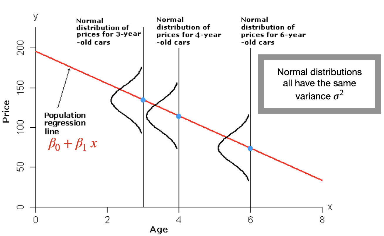
We can see that for each age, the mean price of all cars of that age lies on the regression line \(E(Y|x)=\beta_0+\beta_1x\). And, the prices of all cars of that age are assumed to be normally distributed with mean equal to \(\beta_0+\beta_1 x\) and variance \(\sigma^2\). For example, the prices of all 4-year-old cars must be normally distributed with mean \(\beta_0+\beta_1 (4)\) and variance \(\sigma^2\).
We used the least square method to find the best fit for this data set, and residuals can be obtained as \(e_i=y_i-\hat{y_i}= y_i-(195.47 -20.26x_i)\).
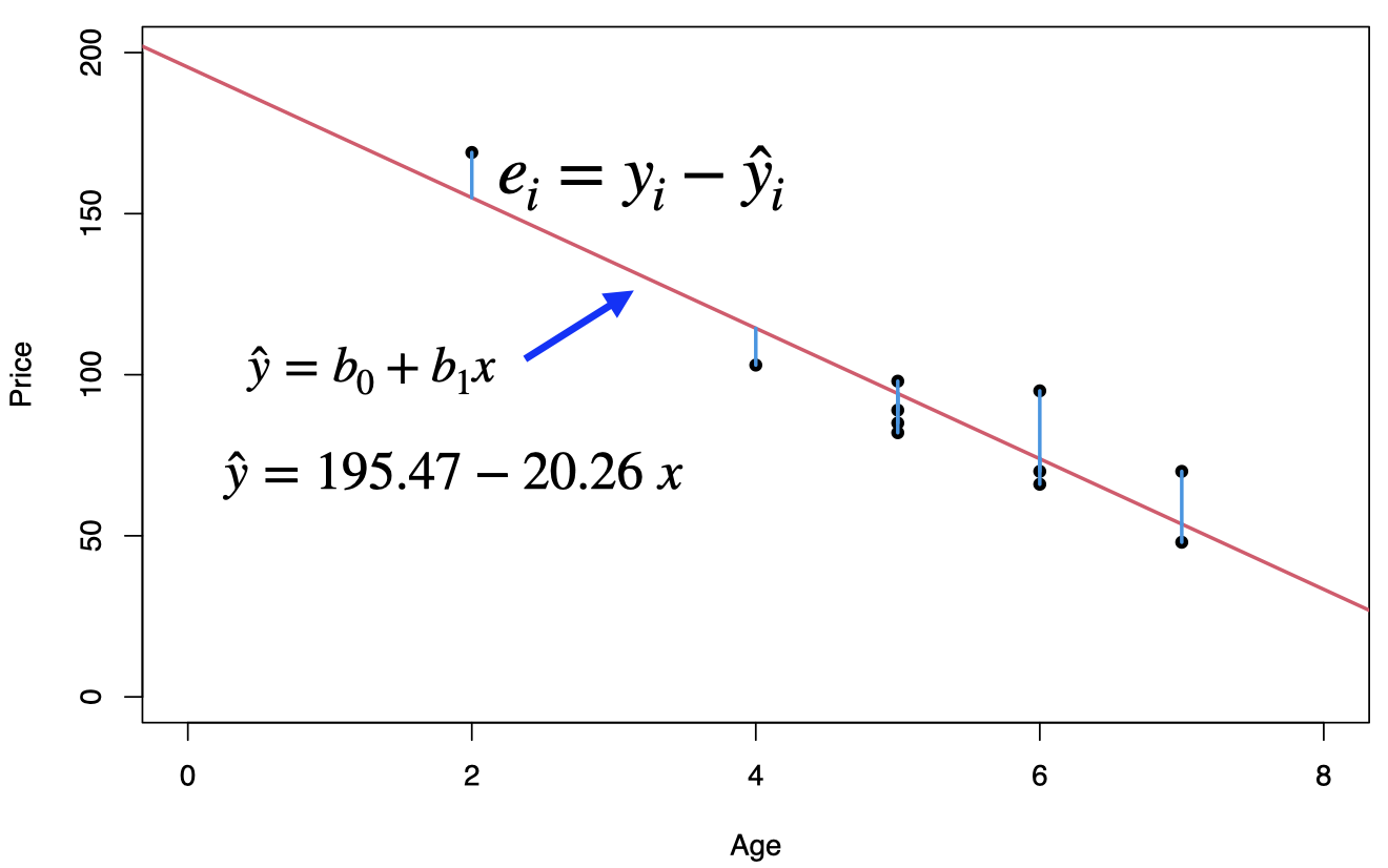
Residual Analysis
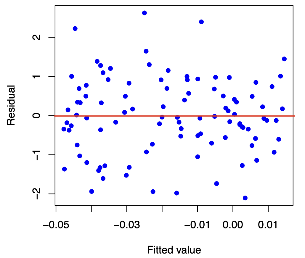
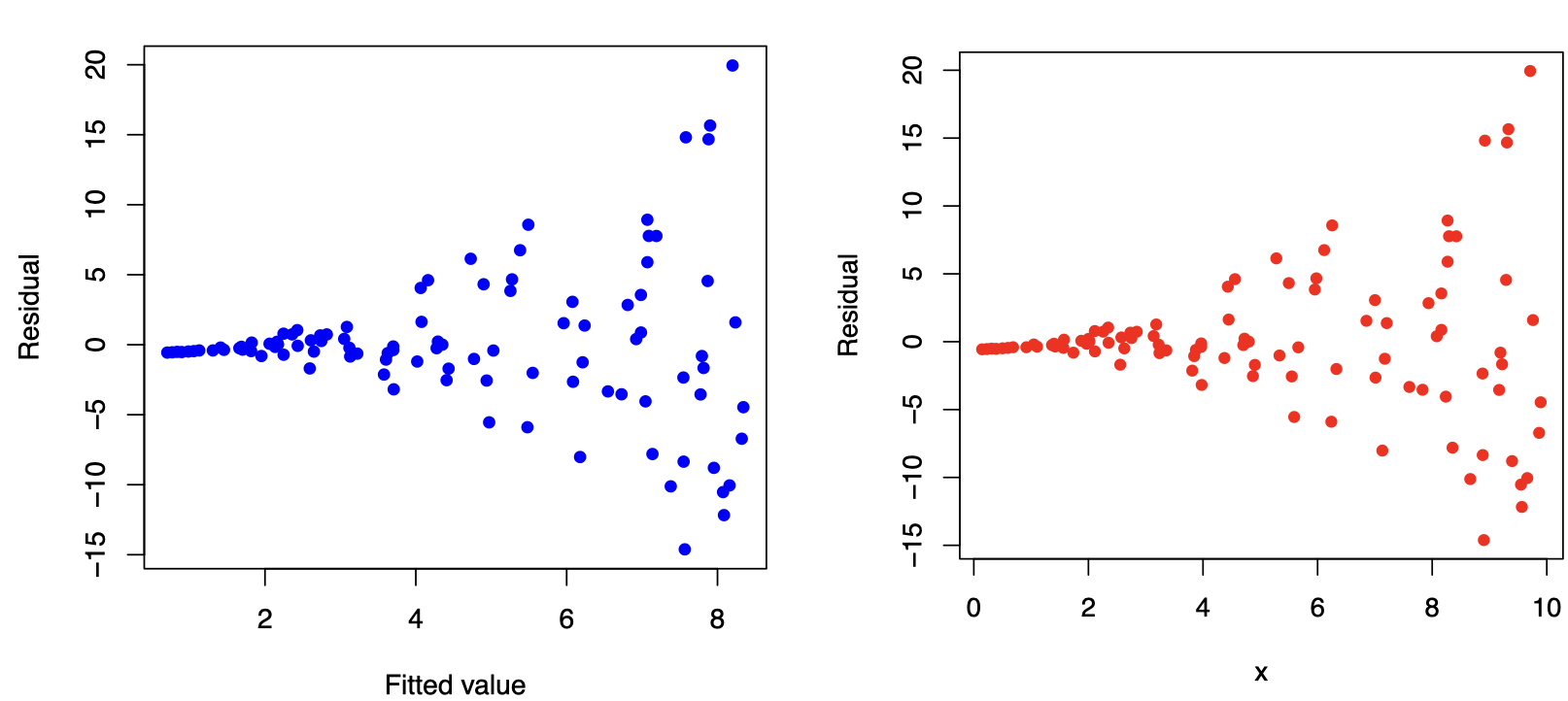
The easiest way to check the simple linear regression assumptions is by constructing a scatterplot of the residuals (\(e_i=y_i-\hat{y_i}\)) against the fitted values (\(\hat{y_i}\)) or against \(x\). If the model is a good fit, then the residual plot should show an even and random scatter of the residuals.
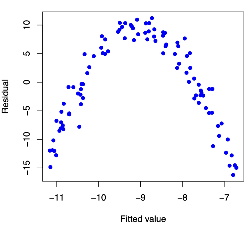
Linearity
The regression needs to be linear in the parameters.
\[Y=\beta_0+\beta_1\;x+\epsilon\] \[E(Y_i|X_i)=\beta_0+\beta_1\;x_i \equiv E(\epsilon_i|X_i)=E(\epsilon_i)=0\]
The residual plot below shows that a linear regression model is not appropriate for this data.
Constant error variance (homoscedasticity)
The plot shows the spread of the residuals is increasing as the fitted values (or \(x\)) increase, which indicates that we have Heteroskedasticity (non-constant variance). The standard errors are biased when heteroskedasticity is present, but the regression coefficients will still be unbiased.
How to detect?
Residuals plot (fitted vs residuals)
Goldfeld–Quandt test
Breusch-Pagan test
How to fix?
White’s standard errors
Weighted least squares model
Taking the log
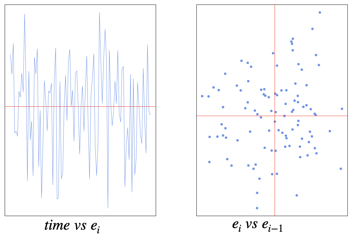
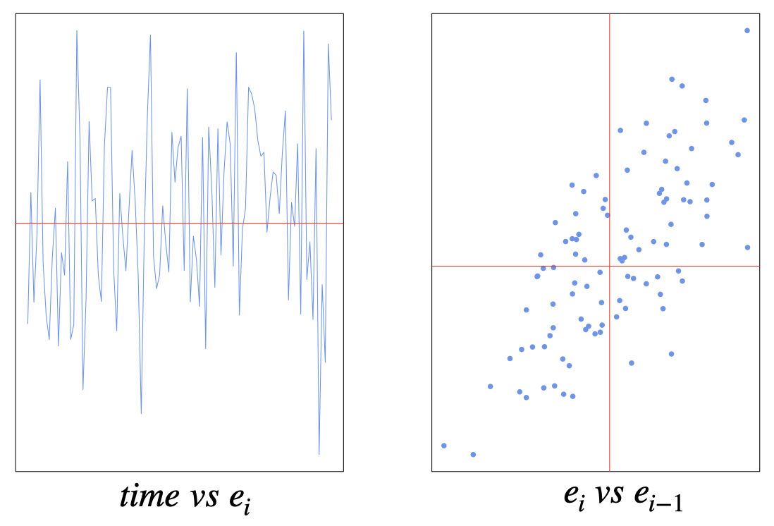
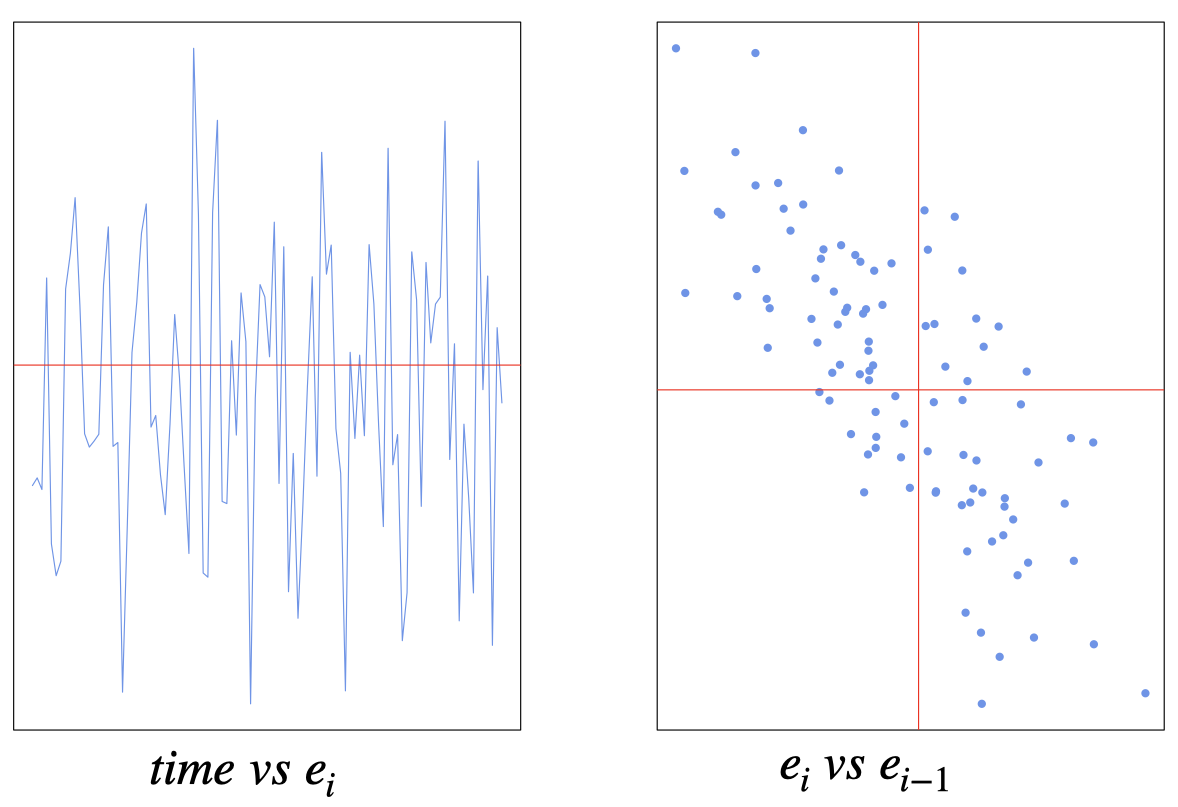
Independent errors terms (no autocorrelation)
The problem of autocorrelation is most likely to occur in time series data, however, it can also occur in cross-sectional data, e.g. if the model is incorrectly specified. When autocorrelation is present, the regression coefficients will still be unbiased, however, the standard errors and test statitics are no longer valid.
An example of no autocorrelation
An example of positive autocorrelation
An example of negative autocorrelation
How to detect?
Residuals plot
Durbin-Watson test
Breusch-Godfrey test
How to fix?
Investigate omitted variables (e.g. trend, business cycle)
Use advanced models (e.g. AR model)
Normality of the errors
We need the errors to be normally distributed. Normality is required for the sampling distributions, hypothesis testing and confidence intervals.
How to detect?
Histogram of residuals
Q-Q plot of residuals
Kolmogorov–Smirnov test
Shapiro–Wilk test
How to fix?
Change the functional form (e.g. taking the log)
Larger sample if possible
Box-Cox Transformation
Normality is an important assumption for many statistical techniques. The Box-Cox transformation transforms our data so that it closely resembles a normal distribution.
Box-Cox transformation applies to a positive response \(y\) with the form
\[ y^{(\lambda)} = \begin{cases} \frac{y^\lambda -1}{\lambda} \qquad \lambda \neq 0,\\ \log{y} \qquad \lambda =0 \end{cases} \] such that \(y^{(\lambda)}\) satisfies the assumptions:
\(E(Y_i^{(\lambda)}|X_i)=\beta_0+\beta_1\;x_i\)
\(Var(Y_i^{(\lambda)}|X_i)=\sigma^2\)
\(Y_1^{(\lambda)},Y_2^{(\lambda)},\ldots,Y_n^{(\lambda)}\) are all independent given \(X_i\).
\(Y_i^{(\lambda)}|X_i\sim N(\beta_0+\beta_1x_i,\;\sigma^2)\)
As usually \(\lambda\) varies over \((-2, 2)\), \(y^{(\lambda)}\) encompasses the reciprocal transformation (\(\lambda=-1\)), log (\(\lambda=0\)), square root (\(\lambda=\frac{1}{2}\)), the original scale (\(\lambda=1\)) and the square transformation (\(\lambda=2\)). If the \(y_i\) are not positive we apply the transformation to \(y_i + \gamma\), where \(\gamma\) is chosen to make all the \(y_i + \gamma\) positive.
The Box-Cox method chooses \(\lambda\) according to the likelihood function. Hint: taking account of the Jacobian of the transformation from \(y^{(\lambda)}\) to \(y\), namely \(y^{\lambda -1}\), the density of \(y_i\) is
\[ f(y_i \big| x_i)=\frac{y_i^{\lambda -1}}{(2\pi\sigma^2)^{\frac{1}{2}}} \exp{\left[-\frac{1}{2\sigma^2} \left(y^{(\lambda)}_i - {x}_i \beta_1-\beta_0 \right)^2\right]} \]
In general, one can simply consider \(\lambda\) as a hyperparameter. In machine learning, hyperparameters are parameters whose values control the learning process and determine the values of model parameters that a learning algorithm ends up learning. The prefix ‘hyper_’ suggests that they are ‘top-level’ parameters that control the learning process and the model parameters that result from it. As a machine learning engineer designing a model, you choose and set hyperparameter values that your learning algorithm will use before the training of the model even begins. For example, in the simple linear regression, we choose the value of \(\lambda\) before estimating the model parameter \(\beta_0\) and \(\beta_1\).
Example: Infant mortality and GDP
Let us investigate the relationship between infant mortality and the wealth of a country. We will use data on 207 countries of the world gathered by the UN in 1998 (the ‘UN’ data set is available from the R package ‘carData’). The data set contains two variables: the infant mortality rate in deaths per 1000 live births, and the GDP per capita in US dollars. There are some missing data values for some countries, so we will remove the missing data before we fit our model.
# install.packages("carData")
library(carData)
data(UN)
options(scipen=999)
# Remove missing data
newUN<-na.omit(UN)
str(newUN)
## 'data.frame': 193 obs. of 7 variables:
## $ region : Factor w/ 8 levels "Africa","Asia",..: 2 4 1 1 5 2 3 8 4 2 ...
## $ group : Factor w/ 3 levels "oecd","other",..: 2 2 3 3 2 2 2 1 1 2 ...
## $ fertility : num 5.97 1.52 2.14 5.13 2.17 ...
## $ ppgdp : num 499 3677 4473 4322 9162 ...
## $ lifeExpF : num 49.5 80.4 75 53.2 79.9 ...
## $ pctUrban : num 23 53 67 59 93 64 47 89 68 52 ...
## $ infantMortality: num 124.5 16.6 21.5 96.2 12.3 ...
## - attr(*, "na.action")= 'omit' Named int [1:20] 4 6 21 35 38 54 67 75 77 78 ...
## ..- attr(*, "names")= chr [1:20] "American Samoa" "Anguilla" "Bermuda" "Cayman Islands" ...fit<- lm(infantMortality ~ ppgdp, data=newUN)
summary(fit)##
## Call:
## lm(formula = infantMortality ~ ppgdp, data = newUN)
##
## Residuals:
## Min 1Q Median 3Q Max
## -31.48 -18.65 -8.59 10.86 83.59
##
## Coefficients:
## Estimate Std. Error t value Pr(>|t|)
## (Intercept) 41.3780016 2.2157454 18.675 < 0.0000000000000002 ***
## ppgdp -0.0008656 0.0001041 -8.312 0.0000000000000173 ***
## ---
## Signif. codes: 0 '***' 0.001 '**' 0.01 '*' 0.05 '.' 0.1 ' ' 1
##
## Residual standard error: 25.13 on 191 degrees of freedom
## Multiple R-squared: 0.2656, Adjusted R-squared: 0.2618
## F-statistic: 69.08 on 1 and 191 DF, p-value: 0.0000000000000173plot(newUN$infantMortality ~ newUN$ppgdp, xlab="GDP per Capita", ylab="Infant mortality (per 1000 births)", pch=16, col="cornflowerblue")
abline(fit,col="red")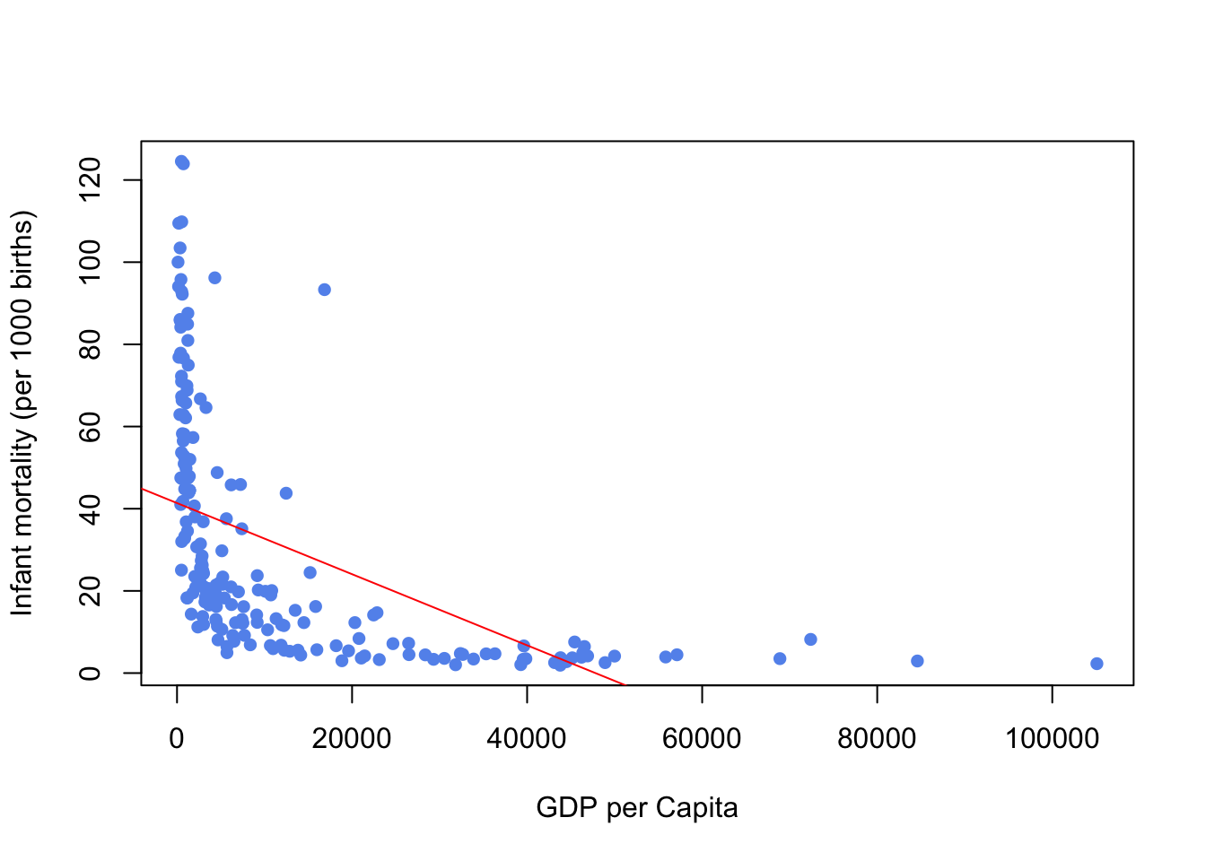
We can see from the scatterplot that the relationship between the two variables is not linear. There is a concentration of data points at small values of GDP (many poor countries) and a concentration of data points at small values of infant mortality (many countries with very low mortality). This suggests a skewness to both variables which would not conform to the normality assumption. Indeed, the regression line (the red line) we construct is a poor fit and only has an \(R^2\) of 0.266.
From the residual plot below we can see a clear evidence of structure to the residuals suggesting the linear relationship is a poor description of the data, and substantial changes in spread suggesting the assumption of homogeneous variance is not appropriate.
# diagnostic plots
plot(fit,which=1,pch=16,col="cornflowerblue")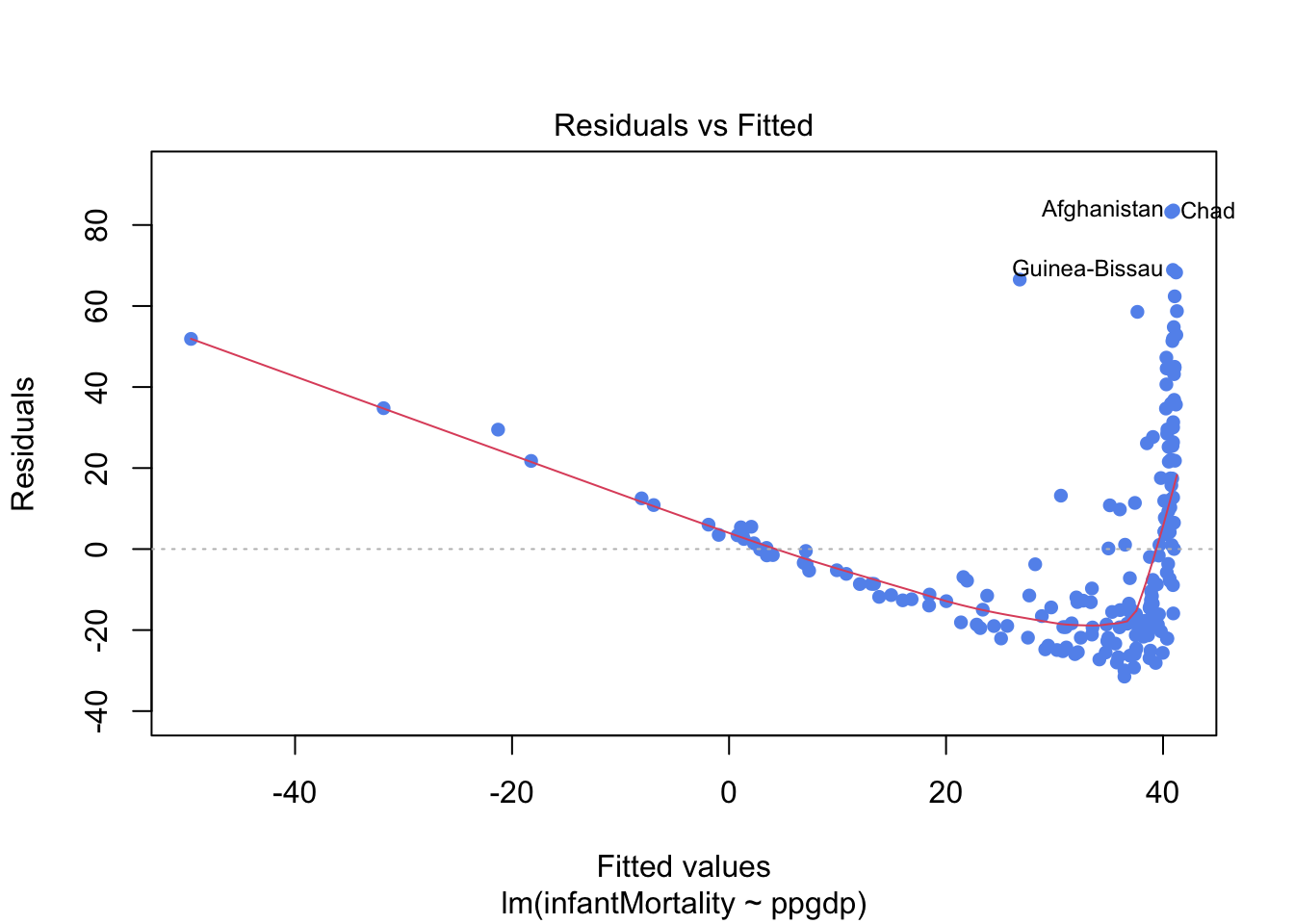
So we can apply a transformation to one or both variables, e.g. taking the log or adding a quadratic form. Notice that this will not affect (violet) the linearity assumption as the regression will still be linear in the parameters. So if we take the logs of both variables gives us the scatterplot of the transformed data set, below, which appears to show a more promising linear structure. The quality of the regression is now improved, with an \(R^2\) value of 0.766, which is still a little weak due to the rather large spread in the data.
fit1<- lm(log(infantMortality) ~ log(ppgdp), data=newUN)
summary(fit1)
##
## Call:
## lm(formula = log(infantMortality) ~ log(ppgdp), data = newUN)
##
## Residuals:
## Min 1Q Median 3Q Max
## -1.16789 -0.36738 -0.02351 0.24544 2.43503
##
## Coefficients:
## Estimate Std. Error t value Pr(>|t|)
## (Intercept) 8.10377 0.21087 38.43 <0.0000000000000002 ***
## log(ppgdp) -0.61680 0.02465 -25.02 <0.0000000000000002 ***
## ---
## Signif. codes: 0 '***' 0.001 '**' 0.01 '*' 0.05 '.' 0.1 ' ' 1
##
## Residual standard error: 0.5281 on 191 degrees of freedom
## Multiple R-squared: 0.7662, Adjusted R-squared: 0.765
## F-statistic: 625.9 on 1 and 191 DF, p-value: < 0.00000000000000022plot(log(newUN$infantMortality) ~ log(newUN$ppgdp), xlab="GDP per Capita", ylab="Infant mortality (per 1000 births)", pch=16, col="cornflowerblue")
abline(fit1,col="red")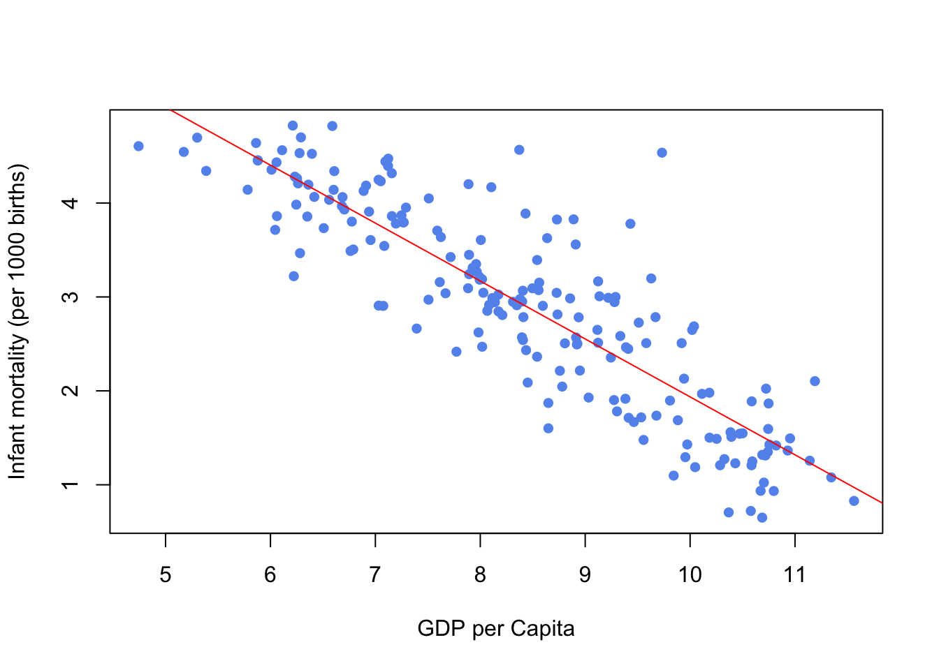
So we check the residuals again, as we can see from the residuals plot below that the log transformation has corrected many of the problems with with residual plot and the residuals now much closer to the expected random scatter.
# diagnostic plots
plot(fit1,which=1,pch=16,col="cornflowerblue")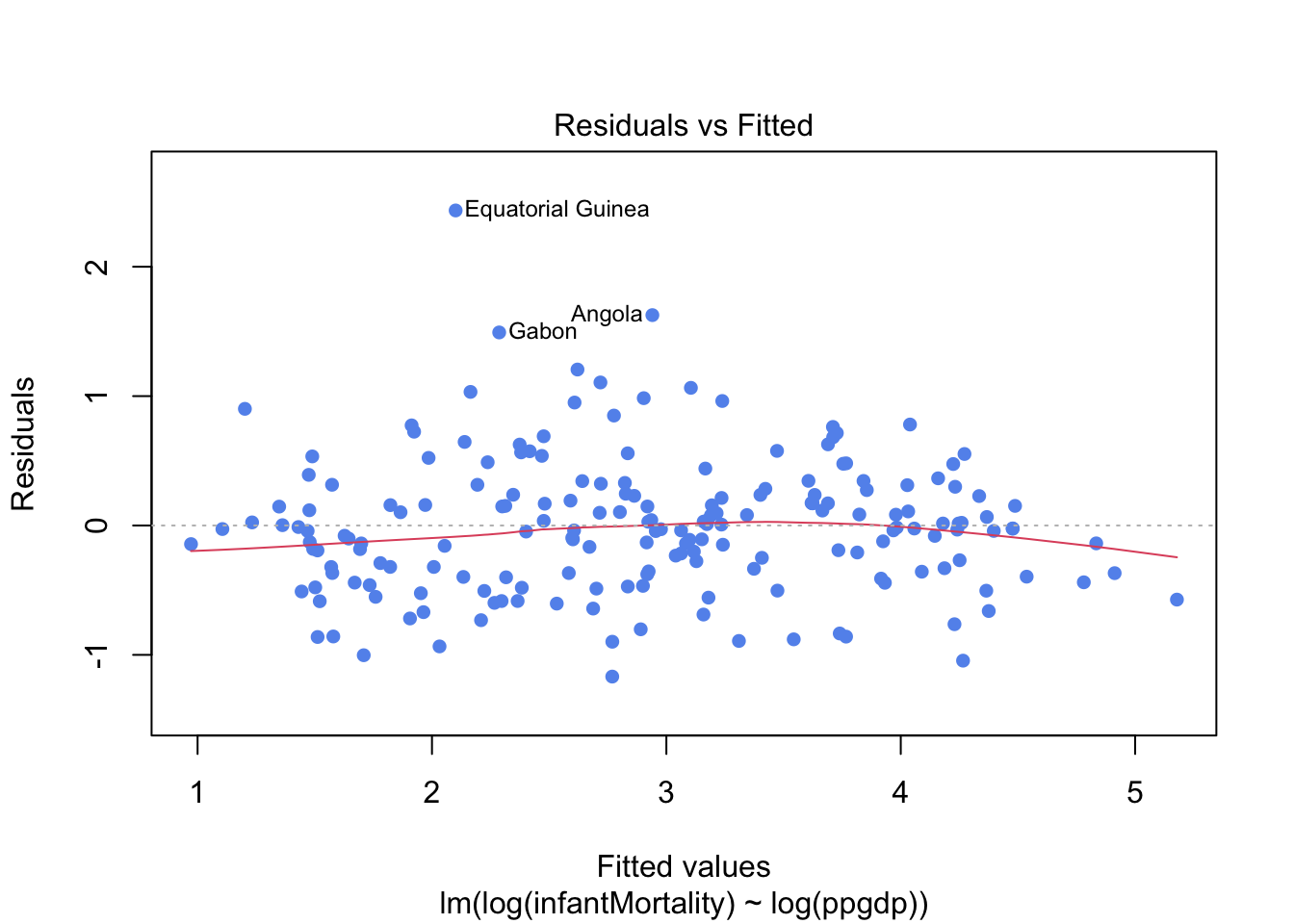
Now let us check the Normality of the errors by creating a histogram and normal QQ plot for the residuals, before and after the log transformation. The normal quantile (QQ) plot shows the sample quantiles of the residuals against the theoretical quantiles that we would expect if these values were drawn from a Normal distribution. If the Normal assumption holds, then we would see an approximate straight-line relationship on the Normal quantile plot.
par(mfrow=c(2,2))
# before the log  transformation.
plot(fit, which = 2,pch=16, col="cornflowerblue")
hist(resid(fit),col="cornflowerblue",main="")
# after the log  transformation.
plot(fit1, which = 2, pch=16, col="hotpink3")
hist(resid(fit1),col="hotpink3",main="")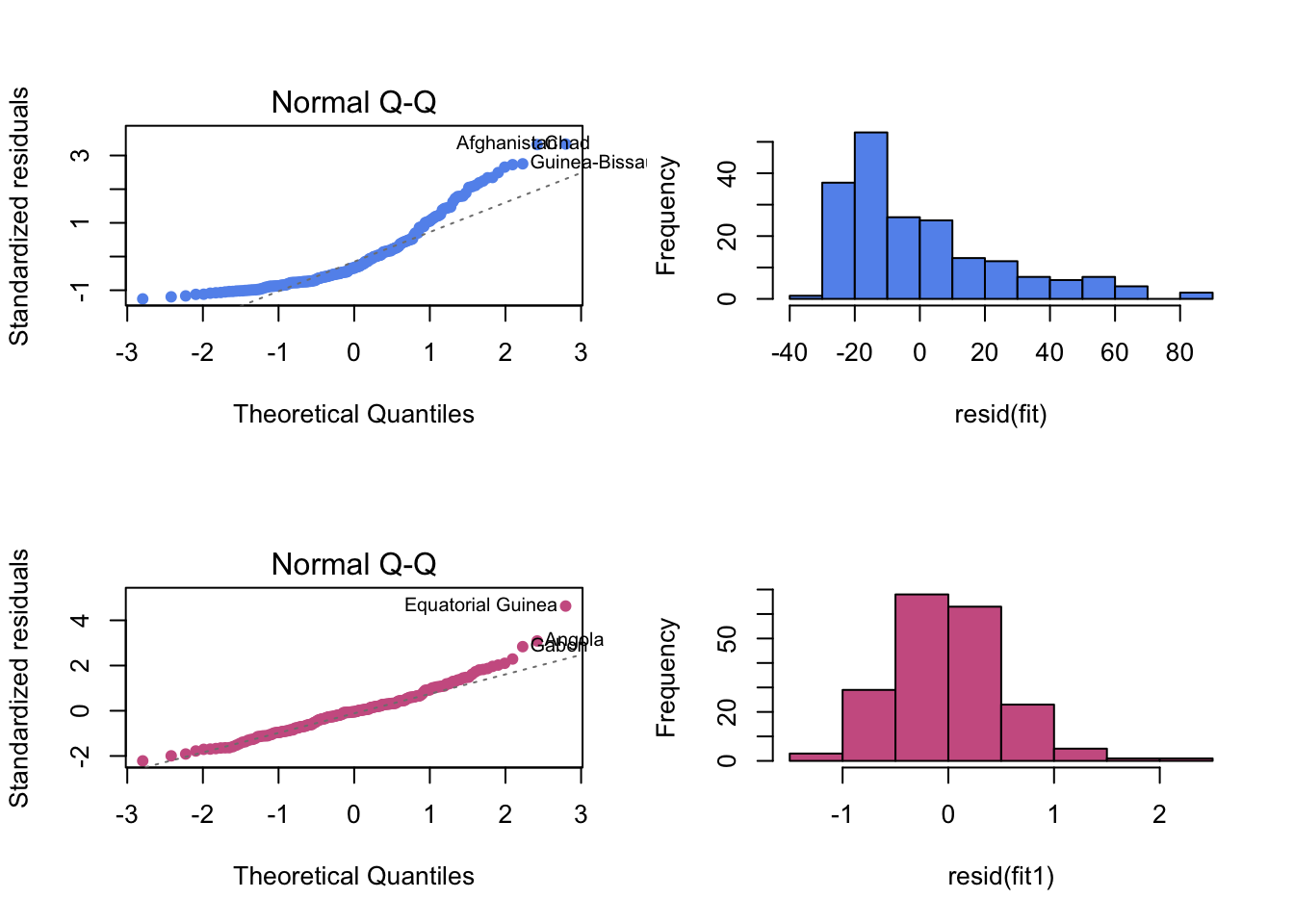
The normal quantile plot and the histogram of residuals (before the log transformation) show strong departure from the expectation of an approximately straight line, with curvature in the tails which reflects the skewness of the data. Finally, the normal quantile plot and the histogram of residuals suggest that residuals are much closer to Normality after the transformation, with some minor deviations in the tails.
3.4 Simple Linear Regression: Inference
Simple Linear Regression Assumptions
Linearity of the relationship between the dependent and independent variables
Independence of the errors (no autocorrelation)
Constant variance of the errors (homoscedasticity)
Normality of the error distribution.
Simple Linear Regression Model
The simple linear regression model for \(Y\) on \(x\) is \[Y=\beta_0+\beta_1 x+\epsilon\] where
\(Y\) : the dependent or response variable
\(x\) : the independent or predictor variable, assumed known
\(\beta_0,\beta_1\) : the regression parameters, the intercept and the slope of the regression line
\(\epsilon\) : the random regression error around the line.
The simple linear regression equation
- The regression equation for a set of \(n\) data points is \(\hat{y}=b_0+b_1\;x\), where \[b_1=\frac{S_{xy}}{S_{xx}}=\frac{\sum (x_i-\bar{x})(y_i-\bar{y})}{\sum (x_i-\bar{x})^2}\] and \[b_0=\bar{y}-b_1\; \bar{x}\]
- \(y\) is the dependent variable (or response variable) and \(x\) is the independent variable (predictor variable or explanatory variable).
- \(b_0\) is called the y-intercept and \(b_1\) is called the slope.
Residual standard error, \(s_e\)
The residual standard error, \(s_e\), is defined by \[s_e=\sqrt{\frac{SSE}{n-2}}\] where \(SSE\) is the error sum of squares (also known as the residual sum of squares, RSS) which can be defined as \[SSE=\sum e^2_i=\sum(y_i-\hat{y}_i)^2=S_{yy}-\frac{S^2_{xy}}{S_{xx}}\] \(s_e\) indicates how much, on average, the observed values of the response variable differ from the predicted values of the response variable. Under the simple linear regression assumptions, \(s_e\) is an unbiased estimate for the error standard deviation \(\sigma\).
Properties of Regression Coefficients
Under the simple linear regression assumptions, the least square estimates \(b_0\) and \(b_1\) are unbiased for the \(\beta_0\) and \(\beta_1\), respectively, i.e.
\(E[b_0]=\beta_0\) and \(E[b_1]=\beta_1\).
The variances of the least squares estimators in simple linear regression are:
\[Var[b_0]=\sigma^2_{b_0}=\sigma^2\left(\frac{1}{n}+\frac{\bar{x}^2}{S_{xx}}\right)\]
\[Var[b_1]=\sigma^2_{b_1}=\frac{\sigma^2}{S_{xx}}\] \[Cov[b_0,b_1]=\sigma_{b_0,b_1}=-\sigma^2\frac{\bar{x}}{S_{xx}}\]
We use \(s_e\) to estimate the error standard deviation \(\sigma\):
\[s^2_{b_0}=s_e^2\left(\frac{1}{n}+\frac{\bar{x}^2}{S_{xx}}\right)\]
\[s^2_{b_1}=\frac{s_e^2}{S_{xx}}\]
\[s_{b_0,b_1}=-s_e^2\frac{\bar{x}}{S_{xx}}\]
The proof of some of the properties are provided in the following, the rest can be find in exercise sheets.
Proof of \(E[b_1]=\beta_1\)
\[\begin{equation} \begin{split} E(b_1) & = E\left(\frac{\sum (x_i-\bar{x})(y_i-\bar{y})}{\sum (x_i-\bar{x})^2}\right)\\ & = E\left(\frac{\sum (x_i-\bar{x})y_i-\bar{y}\sum (x_i-\bar{x}))}{\sum (x_i-\bar{x})^2}\right) \end{split} \end{equation}\] Note \(\sum (x_i-\bar{x})=0\), hence \[\begin{equation} \begin{split} E(b_1) & = E\left(\frac{\sum (x_i-\bar{x})y_i}{\sum (x_i-\bar{x})^2}\right) \\ & = \frac{\sum (x_i-\bar{x})(\beta_0+\beta_1 x_i)}{\sum (x_i-\bar{x})^2}\\ & = \frac{\sum (x_i-\bar{x})\beta_1 x_i}{\sum (x_i-\bar{x})^2} \end{split} \end{equation}\] Note \(\sum (x_i-\bar{x})^2=\sum (x_i-\bar{x})x_i\), hence \[\begin{equation} \begin{split} E(b_1) & = \beta_1 \end{split} \end{equation}\]
Proof of \(Var[b_1]=\frac{\sigma^2}{S_{xx}}\)
From the proof of \(E[b_1]=\beta_1\), we have \[\begin{equation} \begin{split} Var(b_1) & = Var\left(\frac{\sum (x_i-\bar{x})(y_i-\bar{y})}{\sum (x_i-\bar{x})^2}\right)\\ & = Var\left(\frac{\sum (x_i-\bar{x})y_i}{\sum (x_i-\bar{x})^2}\right) \\ & = \frac{Var(\sum (x_i-\bar{x})y_i)}{(\sum (x_i-\bar{x})^2)^2} \\ & = \frac{\sum_{i=1}^{n}Var[ (x_i-\bar{x})y_i]+\sum_{i\neq j}2(x_i-\bar{x})(x_j-\bar{x})Cov(y_i,y_j)}{(\sum (x_i-\bar{x})^2)^2} \end{split} \end{equation}\] Since \(y_i\)s are independent, hence \[\begin{equation} \begin{split} Var(b_1) & = \frac{\sum_{i=1}^{n}Var[ (x_i-\bar{x})y_i]+\sum_{i\neq j}2(x_i-\bar{x})(x_j-\bar{x})Cov(y_i,y_j)}{(\sum (x_i-\bar{x})^2)^2} \\ & = \frac{\sum(x_i-\bar{x})^2\sigma^2}{(\sum (x_i-\bar{x})^2)^2} \\ & =\frac{\sigma^2}{S_{xx}} \end{split} \end{equation}\]
Proof of \(Var[b_0]=\sigma^2\left(\frac{1}{n}+\frac{\bar{x}^2}{S_{xx}}\right)\) \[\begin{equation} \begin{split} Var(b_0) & = Var\left(\bar{y}-b_1 \bar{x}\right)\\ & = Var(\bar{y})+Var(b_1 \bar{x})-2Cov(\bar{y},b_1 \bar{x})\\ & = Var(\frac{\sum y_i}{n})+\bar{x}^2Var(b_1)-2Cov(\bar{y},b_1 \bar{x}) \\ & = = \frac{\sigma^2}{n}+\bar{x}^2\frac{\sigma^2}{S_{xx}}-2Cov(\bar{y},b_1 \bar{x}) \end{split} \end{equation}\] where \[\begin{equation} \begin{split} Cov(\bar{y},b_1 \bar{x})& = Cov\left(\frac{\sum y_i}{n}, \frac{\sum(x_i-\bar{x})y_i}{\sum(x_i-\bar{x})^2}\bar{x}\right)\\ & = \frac{\bar{x}}{n\sum(x_i-\bar{x})^2}Cov[\sum y_i,\sum(x_i-\bar{x})y_i] \end{split} \end{equation}\]
\[\begin{equation} \begin{split} Cov[\sum y_i,\sum(x_i-\bar{x})y_i] & = E[(\sum y_i) \sum(x_i-\bar{x})y_i] -E[\sum y_i]E[\sum(x_i-\bar{x})y_i] \\ & = E[\sum (x_i-\bar{x})y_i^2+\sum_{i\neq j}(x_i-\bar{x})y_iy_j] -nE[y]\sum(x_i-\bar{x})E(y_i) \\ & = \sum (x_i-\bar{x}) (Var(y_i)+E(y_i)^2)+\sum_{i\neq j}(x_i-\bar{x})E(y_i)E(y_j)\\ & -n E[y]^2\sum(x_i-\bar{x}) \\ & =(Var(y)+E(y)^2) \sum (x_i-\bar{x}) +E(y)^2\sum(x_i-\bar{x})\\ & -n E[y]^2\sum(x_i-\bar{x}) \\ & = 0 \end{split} \end{equation}\] Hence \[\begin{equation} \begin{split} Var(b_0) & = \sigma^2\left(\frac{1}{n}+\frac{\bar{x}^2}{S_{xx}}\right) \end{split} \end{equation}\]
Sampling distribution of the least square estimators
For the Normal error simple linear regression model: \[b_0\sim N(\beta_0,\sigma^2_{b_0}) \rightarrow \frac{b_0-\beta_0}{\sigma_{b_0}}\sim N(0,1)\] and \[b_1\sim N(\beta_1,\sigma^2_{b_1}) \rightarrow \frac{b_1-\beta_1}{\sigma_{b_1}}\sim N(0,1)\]
We use \(s_e\) to estimate the error standard deviation \(\sigma\): \[\frac{b_0-\beta_0}{s_{b_0}}\sim t_{n-2}\] and \[\frac{b_1-\beta_1}{s_{b_1}}\sim t_{n-2}\]
Degrees of Freedom
In statistics, degrees of freedom are the number of independent pieces of information that go into the estimate of a particular parameter.
Typically, the degrees of freedom of an estimate of a parameter is equal to the number of independent observations that go into the estimate, minus the number of parameters that are estimated as intermediate steps in the estimation of the parameter itself.
The sample variance has \(n - 1\) degrees of freedom since it is computed from n pieces of data, minus the 1 parameter estimated as the intermediate step, the sample mean. Similarly, having estimated the sample mean we only have \(n - 1\) independent pieces of data left, as if we are given the sample mean and any \(n - 1\) of the observations then we can determine the value of the remaining observation exactly.
\[s^2=\frac{\sum(x_i-\bar{x})^2}{n-1}\]
- In linear regression, the degrees of freedom of the residuals is \(df=n-k^*\), where \(k^*\) is the number of estimated parameters (including the intercept). So for the simple linear regression, we are estimating \(\beta_0\) and \(\beta_1\), thus \(df=n-2\).
Inference for the intercept \(\beta_0\)
Hypotheses:\[H_0:\beta_0=0\;\; \text{against}\;\; H_1:\beta_0\neq 0\]
Test statistic: \[t=\frac{b_0}{s_{b_0}}\] has a t-distribution with \(df=n-2\), where \(s_{b_0}\) is the standard error of \(b_0\), and given by \[s_{b_0}=s_e\sqrt{\frac{1}{n}+\frac{\bar{x}^2}{S_{xx}}}\] and
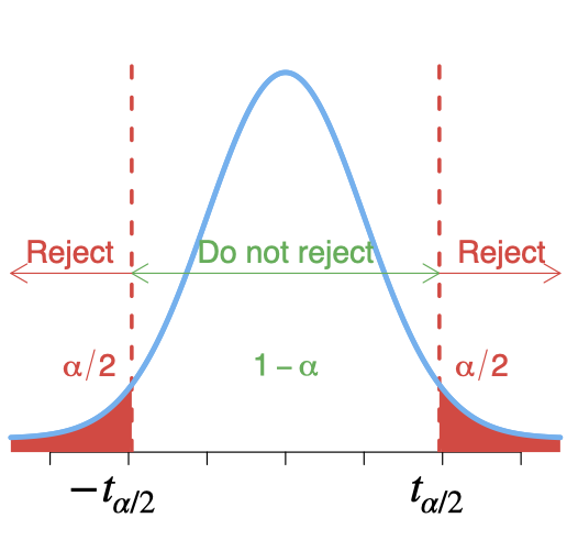
\[s_e=\sqrt{\frac{SSE}{n-2}}=\sqrt{\frac{\sum(y_i-\hat{y}_i)^2}{n-2}}\] We reject \(H_0\) at level \(\alpha\) if \(|t|>t_{\alpha/2}\) with \(df=n-2\).
- 100(1-\(\alpha\))% confidence interval for \(\beta_0\),
\[b_0 \pm t_{\alpha/2} .\;s_{b_0}\] where \(t_{\alpha/2}\) is critical value obtained from the t‐distribution table with \(df=n-2\).
Inference for the slope \(\beta_1\)
Hypotheses: \[H_0:\beta_1=0\;\; \text{against}\;\; H_1:\beta_1\neq 0\]
Test statistic: \[t=\frac{b_1}{s_{b_1}}\] has a t-distribution with \(df=n-2\), where \(s_{b_1}\) is the standard error of \(b_1\),and given by
\[s_{b_1}=\frac{s_e}{\sqrt{S_{xx}}}\]
and
\[s_e=\sqrt{\frac{SSE}{n-2}}=\sqrt{\frac{\sum(y_i-\hat{y}_i)^2}{n-2}}\] We reject \(H_0\) at level \(\alpha\) if \(|t|>t_{\alpha/2}\) with \(df=n-2\).
- 100(1-\(\alpha\))% confidence interval for \(\beta_1\),
\[b_1 \pm t_{\alpha/2} \;s_{b_1}\] where \(t_{\alpha/2}\) is critical value obtained from the t‐distribution table with \(df=n-2\).
Is the regression model “useful”?
Goodness of fit test
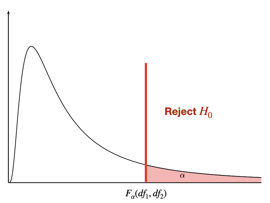
We test the null hypothesis \(H_0:\beta_1=0\) against \(H_1:\beta_1\neq 0\), the F-statistic \[F=\frac{MSR}{MSE}=\frac{SSR}{SSE/(n-2)}\] has F-distribution with degrees of freedom \(df_1=1\) and \(df_2=n-2\).
We reject \(H_0\), at level \(\alpha\), if \(F>F_{\alpha}(df_1,df_2)\).
For a simple linear regression ONLY, F-test is equivalent to t-test for \(\beta_1\).
Regression in R (Used cars example)
Price<-c(85, 103,  70,  82,  89,  98,  66,  95, 169,  70,  48)
Age<- c(5, 4, 6, 5, 5, 5, 6, 6, 2, 7, 7)
carSales<-data.frame(Price,Age)
str(carSales)
## 'data.frame': 11 obs. of 2 variables:
## $ Price: num 85 103 70 82 89 98 66 95 169 70 ...
## $ Age : num 5 4 6 5 5 5 6 6 2 7 ...# simple linear regression
reg<-lm(Price~Age)
summary(reg)##
## Call:
## lm(formula = Price ~ Age)
##
## Residuals:
## Min 1Q Median 3Q Max
## -12.162 -8.531 -5.162 8.946 21.099
##
## Coefficients:
## Estimate Std. Error t value Pr(>|t|)
## (Intercept) 195.47 15.24 12.826 0.000000436 ***
## Age -20.26 2.80 -7.237 0.000048819 ***
## ---
## Signif. codes: 0 '***' 0.001 '**' 0.01 '*' 0.05 '.' 0.1 ' ' 1
##
## Residual standard error: 12.58 on 9 degrees of freedom
## Multiple R-squared: 0.8534, Adjusted R-squared: 0.8371
## F-statistic: 52.38 on 1 and 9 DF, p-value: 0.00004882\(~\)
# To obtain the confidence intervals
confint(reg, level=0.95)
## 2.5 % 97.5 %
## (Intercept) 160.99243 229.94451
## Age -26.59419 -13.92833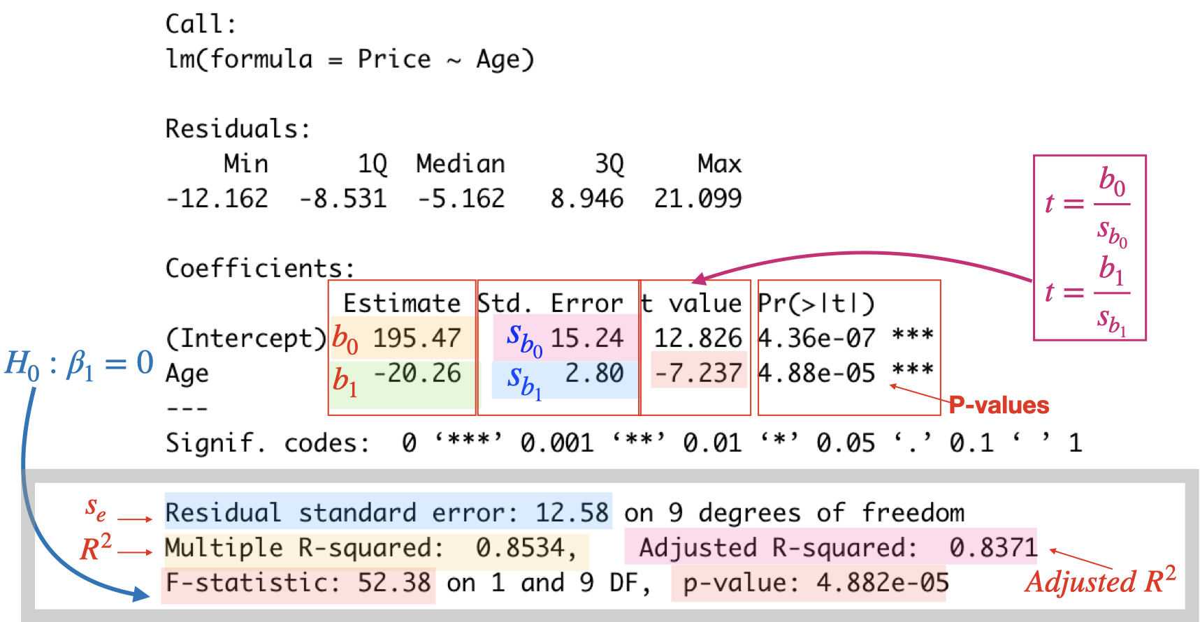
3.5 Simple Linear Regression: Confidence and Prediction intervals
Earlier we introduced simple linear regression as a basic statistical model for the relationship between two random variables. We used the least square method for estimating the regression parameters.
Recall that the simple linear regression model for \(Y\) on \(x\) is \[Y=\beta_0+\beta_1 x+\epsilon\] where
\(Y\) : the dependent or response variable
\(x\) : the independent or predictor variable, assumed known
\(\beta_0,\beta_1\) : the regression parameters, the intercept and the slope of the regression line
\(\epsilon\) : the random regression error around the line.
and the regression equation for a set of \(n\) data points is \(\hat{y}=b_0+b_1\;x\), where \[b_1=\frac{S_{xy}}{S_{xx}}=\frac{\sum (x_i-\bar{x})(y_i-\bar{y})}{\sum (x_i-\bar{x})^2}\] and \[b_0=\bar{y}-b_1\; \bar{x}\] where \(b_0\) is called the y-intercept and \(b_1\) is called the slope.
\(~\)
Under the simple linear regression assumptions, the residual standard error \(s_e\) is an unbiased estimate for the error standard deviation \(\sigma\), where
\[s_e=\sqrt{\frac{SSE}{n-2}}=\sqrt{\frac{\sum(y_i-\hat{y}_i)^2}{n-2}} \] \(s_e\) indicates how much, on average, the observed values of the response variable differ from the predicted values of the response variable.
\(~\)
Below we will see how we can use these least square estimates for prediction. First, we will consider the inference for the conditional mean of the response variable \(y\) given a particular value of the independent variable \(x\), let us call this particular value \(x^*\). Next, we will see how to predict the value of the response variable \(Y\) for a given value of the independent variable \(x^*\). For these confidence and predictive intervals, to be valid, the usual four simple regression assumptions must hold.
Inference for the regression line \(E\left[Y|x^*\right]\)
Suppose we are interested in the value of the regression line at a new point \(x^*\). Let’s denote the unknown true value of the regression line at \(x=x^*\) as \(\mu^*\). From the form of the regression line equation we have
\[\mu^*=\mu_{Y|x^*}=E\left[Y|x^*\right]=\beta_0+\beta_1 x^*\]
but \(\beta_0\) and \(\beta_1\) are unknown. We can use the least square regression equation to estimate the unknown true value of the regression line, so we have
\[\hat{\mu}^*=b_0+b_1 x^*=\hat{y}^*\]
This is simply a point estimate for the regression line. However, in statistics, a point estimate is often not enough, and we need to express our uncertainty about this point estimate, and one way to do so is via confidence interval.
A \(100(1-\alpha)\%\) confidence interval for the conditional mean \(\mu^*\) is \[\hat{y}^*\pm t_{\alpha/2}\;\cdot s_e\;\sqrt{\frac{1}{n}+\frac{(x^*-\bar{x})^2}{S_{xx}}}\] where \(S_{xx}=\sum_{i=1}^{n} (x_i-\bar{x})^2\), and \(t_{\alpha/2}\) is the \(\alpha/2\) critical value from the t-distribution with \(df=n-2\).
Inference for the response variable \(Y\) for a given \(x=x^*\)
Suppose now we are interested in predicting the value of \(Y^*\) if we have a new observation at \(x^*\).
At \(x=x^*\), the value of \(Y^*\) is unknown and given by \[Y^*=\beta_0+\beta_1 x^*+\epsilon\] where but \(\beta_0\), \(\beta_1\) and \(\epsilon\) are unknown. We will use \(\hat{y}^*=b_0+b_1\;x^*\) as a basis for our prediction.
\(~\)
A \(100(1-\alpha)\%\) prediction interval for \(Y^*\) at \(x=x^*\) is
\[\hat{y}^* \pm t_{\alpha/2}\;\cdot s_e\;\sqrt{1+\frac{1}{n}+\frac{(x^*-\bar{x})^2}{S_{xx}}}\] The extra ’1’ under the square root sign, we have here accounts for the extra variability of a single observation about the mean.
Used cars example
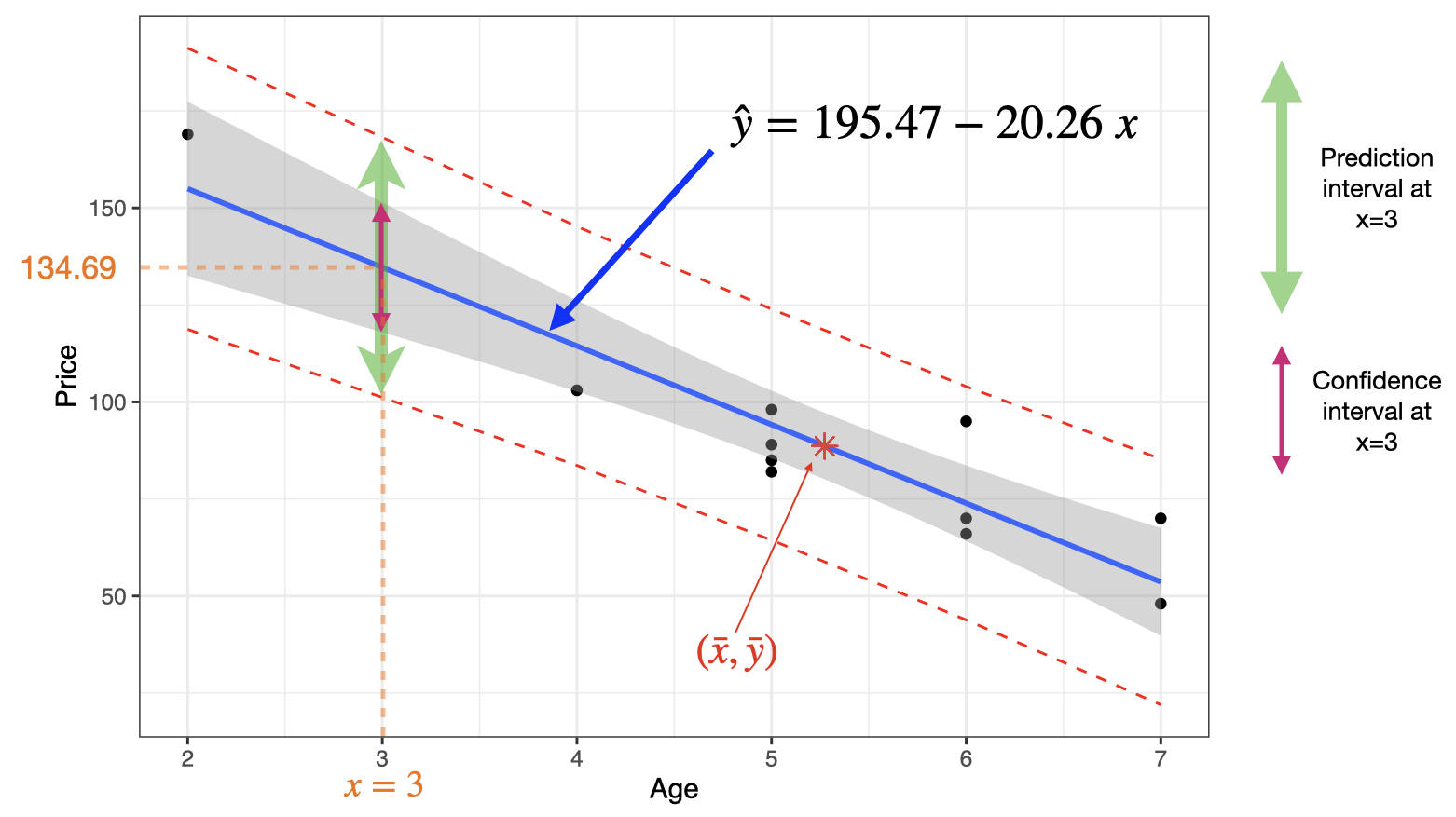
Estimate the mean price of all 3-year-old cars, \(E[Y|x=3]\):
\[\hat{\mu}^*=195.47-20.26 (3)= 134.69=\hat{y}^*\]
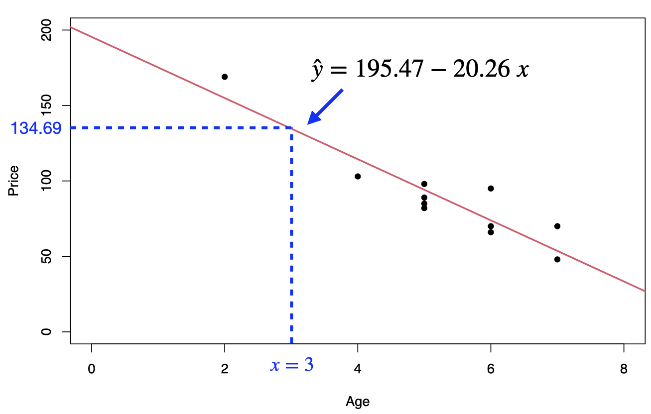
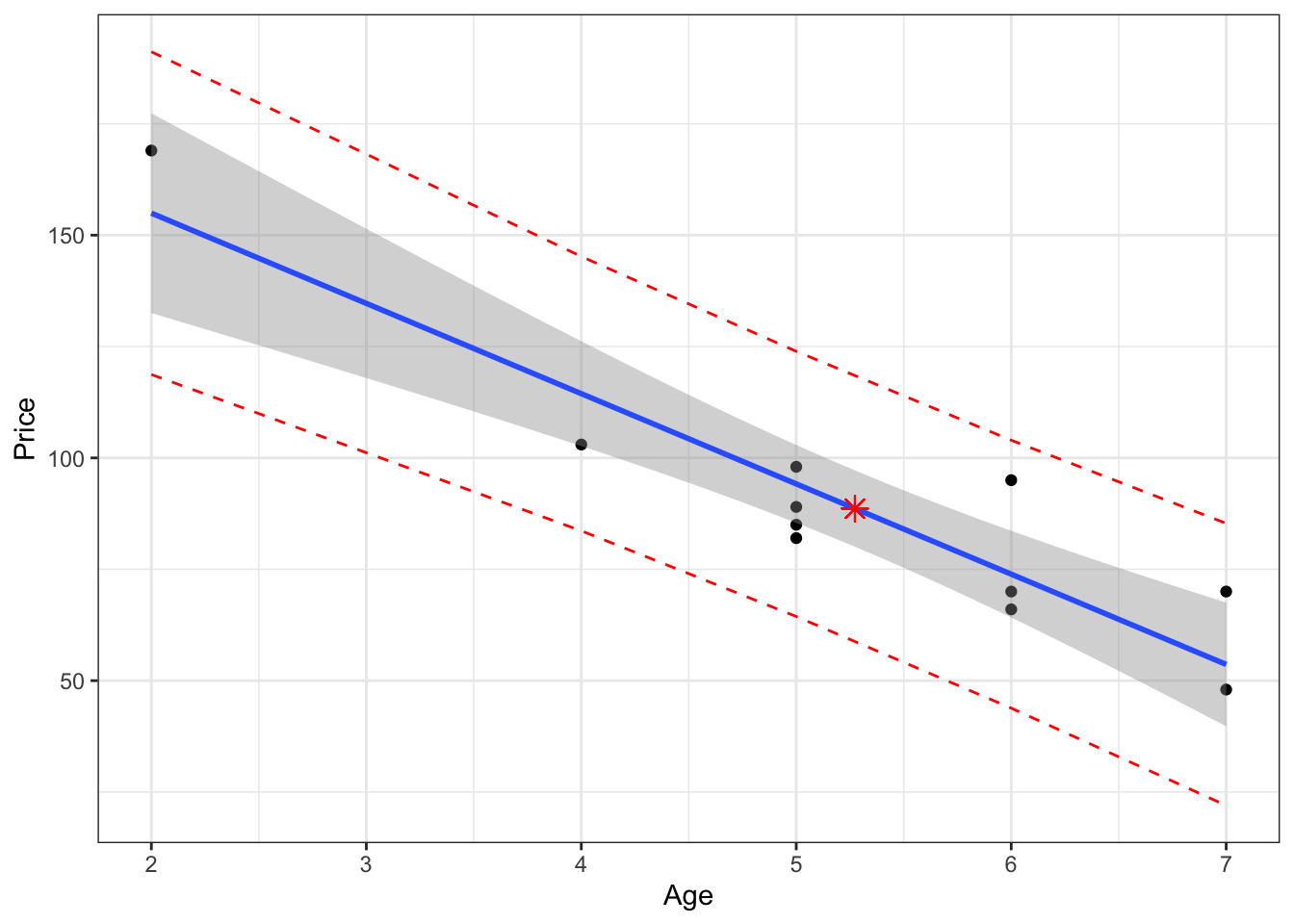
A 95% confidence interval for the mean price of all 3-year-old cars is \[\hat{y}^*\pm t_{\alpha/2}\;\times se\sqrt{\frac{1}{n}+\frac{(x^*-\bar{x})^2}{S_{xx}}}\] \[[195.47-20.26(3)]\pm 2.262\times12.58\sqrt{\frac{1}{11}+\frac{(3-5.273)^2}{(11-1)\times2.018}}\] \[134.69\pm 16.76\] that is \[117.93<\mu^*<151.45\]
Predict the price of a 3-year-old car, \(Y|x=3\): \[\hat{y}^*=195.47-20.26 (3)= 134.69\]
A 95% predictive interval for the price of a 3-year-old car is
\[\hat{y}^*\pm t_{\alpha/2}\;\times se\sqrt{1+\frac{1}{n}+\frac{(x^*-\bar{x})^2}{S_{xx}}}\] \[[195.47-20.26(3)]\pm 2.262\times12.58\sqrt{1+\frac{1}{11}+\frac{(3-5.273)^2}{(11-1)*\times2.018}}\] \[134.69\pm 33.025\] that is \[101.67<Y^*<167.72\]
where \(S_{xx}=\sum_{i=1}^{n} (x_i-\bar{x})^2=(n-1) Var(x)\).
Regression in R
# Build linear model
Price<-c(85, 103,  70,  82,  89,  98,  66,  95, 169,  70,  48)
Age<- c(5, 4, 6, 5, 5, 5, 6, 6, 2, 7, 7)
carSales<-data.frame(Price=Price,Age=Age)

reg <- lm(Price~Age,data=carSales)
summary(reg)
##
## Call:
## lm(formula = Price ~ Age, data = carSales)
##
## Residuals:
## Min 1Q Median 3Q Max
## -12.162 -8.531 -5.162 8.946 21.099
##
## Coefficients:
## Estimate Std. Error t value Pr(>|t|)
## (Intercept) 195.47 15.24 12.826 0.000000436 ***
## Age -20.26 2.80 -7.237 0.000048819 ***
## ---
## Signif. codes: 0 '***' 0.001 '**' 0.01 '*' 0.05 '.' 0.1 ' ' 1
##
## Residual standard error: 12.58 on 9 degrees of freedom
## Multiple R-squared: 0.8534, Adjusted R-squared: 0.8371
## F-statistic: 52.38 on 1 and 9 DF, p-value: 0.00004882mean(Age)## [1] 5.272727var(Age)## [1] 2.018182qt(0.975,9)## [1] 2.262157newage<- data.frame(Age = 3)
predict(reg, newdata = newage, interval = "confidence")## fit lwr upr
## 1 134.6847 117.9293 151.4401predict(reg, newdata = newage, interval = "prediction")## fit lwr upr
## 1 134.6847 101.6672 167.7022\(~\)
We can plot the confidence and prediction intervals as follows:
3.6 Multiple Linear Regression: Introduction
Multiple linear regression model
In simple linear regression, we have one dependent variable (\(y\)) and one independent variable (\(x\)). In multiple linear regression, we have one dependent variable (\(y\)) and several independent variables (\(x_1,x_2, \ldots,x_k\)).
The multiple linear regression model, for the population, can be expressed as \[Y=\beta_0+\beta_1 x_1 +\beta_2 x_2+\ldots+\beta_kx_k+ \epsilon\] where \(\epsilon\) is the error term.
Or using the matrix notation for a sample of \(n\) observations:
\[\begin{bmatrix} y_1 \\ \vdots \\ \vdots \\ y_n \end{bmatrix} = \begin{bmatrix}1 & x_{1,1} & \dots & x_{1,k} \\ 1 & x_{2,1} & \dots & x_{2,k}\\ \vdots & \vdots & \vdots & \vdots \\ 1 & x_{n,1} & \dots & x_{n,k} \end{bmatrix}\begin{bmatrix} \beta_0 \\ \beta_1 \\ \vdots \\ \beta_k \end{bmatrix}+\begin{bmatrix} \epsilon_1 \\ \vdots \\ \vdots \\ \epsilon_n \end{bmatrix} \]
i.e.
\[ \bf{Y}=\bf{X} \boldsymbol{\beta}+\bf{\epsilon} \] where [\(\bf{Y}^T\)] \(=(y_1,\dots,y_n)\) is the vector of responses; [\(\bf{ X}^{}\)], is the design matrix; [\(\boldsymbol{ \beta}^T\)] \(=(\beta_0,\beta_1,\dots,\beta_k)\) is the \(k+1\) dimensional parameter vector; [\(\bf{ \epsilon}^T\)] \(=(\epsilon_1, \dots, \epsilon_n)\) is the vector of errors.
- The corresponding least square estimate, from the sample, of this multiple linear regression model is given by \[\hat{y}=\hat{\beta}_0+\hat{\beta}_1 x_1+\hat{\beta}_2 x_2+\ldots+\hat{\beta}_k x_k\] The LS estimator \(\hat{\boldsymbol{\beta}}=\left(\bf X^{\text{T}}\bf X\right)^{-1} \bf X^{\text{T}}\bf Y\)
- The coefficient \(b_0\) (or \(\hat{\beta}_0\)) represents the \(y\)-intercept, that is, the value of \(y\) when \(x_1=x_2= \ldots=x_k=0\). The coefficient \(b_i\) (or \(\hat{\beta}_i\)) \((i=1, \ldots, k)\) is the partial slope of \(x_i\), holding all other \(x\)’s fixed. So \(b_i\) (or \(\hat{\beta}_i\)) tells us the change in \(y\) for a unit increase in \(x_i\), holding all other \(x\)’s fixed.
Used cars example
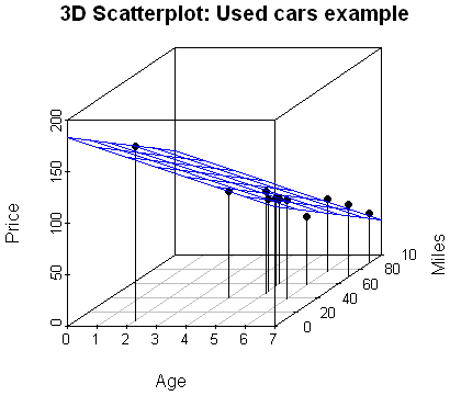
The table below displays data on Age, Miles and Price for a sample of cars of a particular make and model.
| Price (\(y\)) | Age (\(x_1\)) | Miles (\(x_2\)) |
|---|---|---|
| 85 | 5 | 57 |
| 103 | 4 | 40 |
| 70 | 6 | 77 |
| 82 | 5 | 60 |
| 89 | 5 | 49 |
| 98 | 5 | 47 |
| 66 | 6 | 58 |
| 95 | 6 | 39 |
| 169 | 2 | 8 |
| 70 | 7 | 69 |
| 48 | 7 | 89 |
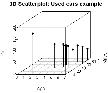

The scatterplot and the correlation matrix show a fairly negative relationship between the price of the car and both independent variables (age and miles). It is desirable to have a relationship between each independent variable and the dependent variable. However, the scatterplot also shows a positive relationship between the age and the miles, which is undesirable as it will cause the issue of Multicollinearity.
Coefficient of determination, \(R^2\) and adjusted \(R^2\)
Recall that \(R^2\) is a measure of the proportion of the total variation in the observed values of the response variable that is explained by the multiple linear regression in the \(k\) predictor variables \(x_1, x_2, \ldots, x_k\).
\(R^2\) will increase when an additional predictor variable is added to the model. One should not simply select a model with many predictor variables because it has the highest \(R^2\) value, it is often good to have a model with a high \(R^2\) value but only a few x’s included.
Adjusted \(R^2\) is a modification of \(R^2\) that takes into account the number of predictor variables. \[\mbox{Adjusted-}R^2=1-(1-R^2)\frac{n-1}{n-k-1}\]
The residual standard error, \(s_e\)
- Recall that, \[\text{Residual} = \text{Observed value} - \text{Predicted value.}\]
\[e_i=y_i-\hat{y}_i\]
In a multiple linear regression with \(k\) predictors, the standard error of the estimate, \(s_e\), is defined by \[s_e=\sqrt{\frac{SSE}{n-(k+1)}}\;\;\;\;\; \text{where}\;\;SSE=\sum (y_i-\hat{y}_i)^2\]
The standard error of the estimate, \(s_e\), indicates how much, on average, the observed values of the response variable differs from the predicted values of the response variable. The \(s_e\) is the estimate of the common standard deviation \(\sigma\).
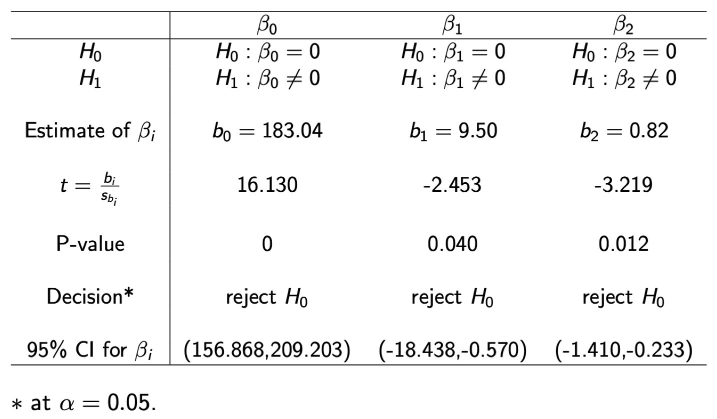
Inferences about a particular predictor variable
To test whether a particular predictor variable, say \(x_i\), is useful for predicting \(y\) we test the null hypothesis \(H_0:\beta_i=0\) against \(H_1:\beta_i\neq 0\).
The test statistic \[t=\frac{b_i}{s_{b_i}}\] has a \(t\)-distribution with degrees of freedom \(df=n-(k+1)\). So we reject \(H_0\), at level \(\alpha\), if \(|t|>t_{\alpha/2}.\)
Rejection of the null hypothesis indicates that \(x_i\) is useful as a predictor for \(y\). However, failing to reject the null hypothesis suggests that \(x_i\) may not be useful as a predictor of \(y\), so we may want to consider removing this variable from the regression analysis.
100(1-\(\alpha\))% confidence interval for \(\beta_i\) is \[b_i \pm t_{\alpha/2} . s_{b_i}\] where \(s_{b_i}\) is the standard error of \(b_i\).
Is the multiple regression model “useful”?
Goodness of fit test
To test how useful is this model, we test the null hypothesis
\(H_0: \beta_1=\beta_2=\ldots =\beta_k=0\), against
\(H_1: \text{at least one of the} \;\beta_i \text{'s is not zero}\). - The \(F\)-statistic \[F=\frac{MSR}{MSE}=\frac{SSR/k}{SSE/(n-k-1)}\] with degrees of freedom \(df_1=k\) and \(df_2=n-(k+1)\).
We reject \(H_0\), at level \(\alpha\), if \(F>F_{\alpha}(df_1,df_2)\).
Used cars example continued
Multiple regression equation: \(\hat{y}=183.04-9.50 x_1- 0.82 x_2\)
The predicted price for a 4-year-old car that has driven 45 thousand miles is \[\hat{y}=183.04-9.50 (4)- 0.82 (45)=108.14\] (as units of $100 were used, this means $10814)
Extrapolation: we need to look at the region (all combined values) not only the range of the observed values of each predictor variable separately.
Regression in R
Price<-c(85, 103,  70,  82,  89,  98,  66,  95, 169,  70,  48)
Age<- c(5, 4, 6, 5, 5, 5, 6, 6, 2, 7, 7)
Miles<-c(57,40,77,60,49,47,58,39,8,69,89)
carSales<-data.frame(Price=Price,Age=Age,Miles=Miles)


# Scatterplot matrix
# Customize upper panel
upper.panel<-function(x, y){
  points(x,y, pch=19, col=4)
  r <- round(cor(x, y), digits=3)
  txt <- paste0("r = ", r)
  usr <- par("usr"); on.exit(par(usr))
  par(usr = c(0, 1, 0, 1))
  text(0.5, 0.9, txt)
}
pairs(carSales, lower.panel = NULL,
      upper.panel = upper.panel)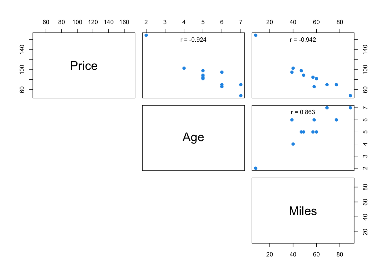
reg <- lm(Price~Age+Miles,data=carSales)
summary(reg)
##
## Call:
## lm(formula = Price ~ Age + Miles, data = carSales)
##
## Residuals:
## Min 1Q Median 3Q Max
## -12.364 -5.243 1.028 5.926 11.545
##
## Coefficients:
## Estimate Std. Error t value Pr(>|t|)
## (Intercept) 183.0352 11.3476 16.130 0.000000219 ***
## Age -9.5043 3.8742 -2.453 0.0397 *
## Miles -0.8215 0.2552 -3.219 0.0123 *
## ---
## Signif. codes: 0 '***' 0.001 '**' 0.01 '*' 0.05 '.' 0.1 ' ' 1
##
## Residual standard error: 8.805 on 8 degrees of freedom
## Multiple R-squared: 0.9361, Adjusted R-squared: 0.9201
## F-statistic: 58.61 on 2 and 8 DF, p-value: 0.00001666confint(reg, level=0.95)## 2.5 % 97.5 %
## (Intercept) 156.867552 209.2028630
## Age -18.438166 -0.5703751
## Miles -1.409991 -0.2329757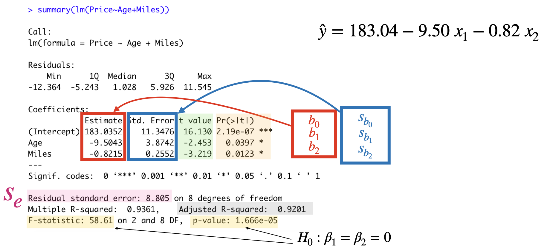
Multiple Linear Regression Assumptions
Linearity: For each set of values, \(x_1, x_2, \ldots, x_k\), of the predictor variables, the conditional mean of the response variable \(y\) is \(\beta_0+\beta_1 x_1+\beta_2 x_2+ \ldots+ \beta_k x_k\).
Equal variance (homoscedasticity): The conditional variance of the response variable are the same (equal to \(\sigma^2\)) for all sets of values, \(x_1, x_2, \ldots, x_k\), of the predictor variables.
Independent observations: The observations of the response variable are independent of one another.
Normally: For each set values, \(x_1, x_2, \ldots, x_k\), of the predictor variables, the conditional distribution of the response variable is a normal distribution.
No Multicollinearity: Multicollinearity exists when two or more of the predictor variables are highly correlated.
Multicollinearity
Multicollinearity refers to a situation when two or more predictor variables in our multiple regression model are highly (linearly) correlated.
The least square estimates will remain unbiased, but unstable.
The standard errors (of the affected variables) are likely to be high.
Overall model fit (e.g. R-square, F, prediction) is not affected.
Multicollinearity: Detect
Scatterplot Matrix
Variance Inflation Factors: the Variance Inflation Factors (VIF) for the \(i^{th}\) predictor is \[VIF_i=\frac{1}{1-R^2_i}\] where \(R^2_i\) is the R-square value obtained by regressing the \(i^{th}\) predictor on the other predictor variables.
\(VIF=1\) indicates that there is no correlation between \(i^{th}\) predictor variable and the other predictor variables.
As a rule of thumb if \(VIF>10\) then multicollinearity could be a problem.
Regression in R (regression assumptions)
plot(reg, which=1, pch=19, col=4)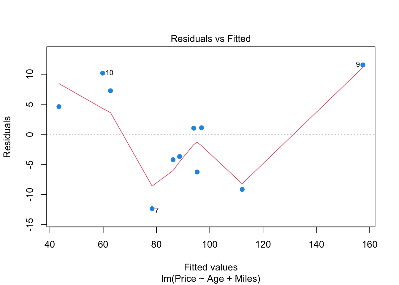
plot(reg, which=2, pch=19, col=4)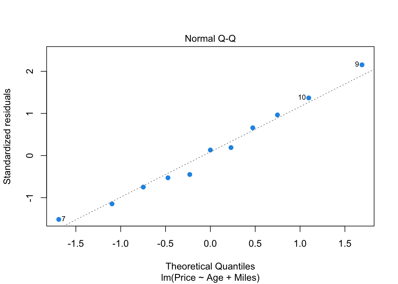
# install.packages("car")
library(car)
vif(reg)
## Age Miles
## 3.907129 3.907129The value of \(VIF=3.91\) indicates a moderate correlation between the age and the miles in the model, but this is not a major concern.