Chapter 6 Shrinkage Methods

6.1 Motivation

Issue due to multicollinearity

Recall that multicollinearity refers to a situation when two or more predictor variables in the linear regression model are highly (linearly) correlated. The least square estimates will become “unstable”. Here we explore the issue via the following simulation study.

This is a simulation study because we simulate data based on a known model, add some random noise, and then investigate how different methods use this data to estimate the regression parameters. We can then evaluate the performance of the method based on how close the estimated parameter values are to the true values.

We assume a correct model of \[y=x_1-x_2+\epsilon\] so that we have true generating \(\beta_0=0\), \(\beta_1=1\) and \(\beta_2 = -1\), and noise term \(\epsilon\sim\mathcal{N}(0,1)\). In other words, for any specified \((x_1,x_2)\), we evaluate the response \(x_1-x_2\) before adding random noise.

Rather than sampling the training data independently, however, we assume a high level of collinearity between \(x_1\) and \(x_2\) by simulating \(x_1\sim\mathcal{N}(0,1)\) and \(x_2\sim\mathcal{N}(0.9x_1,0.2^2)\). In other words, \(x_2\) is a scaling of \(x_1\) with just a small amount of random noise added - there is definitely a strong correlation between the values of those predictors!

Feel free to look through the following code to understand how the simulation study is working and the plots below are generated! Note that \((X^TX)^{-1}X^TY\) is the regression coefficient estimates for LS.

# Number of iterations for the simulation study.
iter <- 50

# Number of training points.
n <- 10

# Empty matrix of NAs for the regression coefficients for LS 
b_LS <- matrix( NA, nrow = 2, ncol = iter )


# For each iteration...
for( i in 1:iter ){

  # As we can see x2 is highly correlated with x1 - COLLINEARITY!
  x1 <- rnorm( n )
  x2 <- 0.9 * x1 + rnorm( n, 0, 0.2 )
  
  # Design matrix.
  x <- cbind( x1, x2 )
  
  # y = x1 - x2 + e, where error e is N(0,1)
  y <- x1 - x2 + rnorm( n )
  
  # LS regression components - the below calculation obtains them given the 
  # training data and response generated in this iteration, and stores 
  # those estimates in the relevant column of the matrix b_LS.
  b_LS[,i]<- solve( t(x) %*% x ) %*% t(x) %*% y
  

}

# Now we plot the results.  

# Plot the LS estimates for beta_1.
plot( b_LS[1,], col = 'blue', pch = 16, ylim = c( min(b_LS), max(b_LS) ),
      ylab = 'Estimated coefficients', xlab = 'Least squares', bty ='l' )
# Add the LS estimates for beta_2 in a different colour.
points( b_LS[2,], col = 'red', pch = 17 )
# Add horizontal lines representing the true values of beta_1 and beta_2.
abline( a = 1, b = 0, col = 'blue' ) # Plot the true value of beta_1 = 1.
abline( a = -1, b = 0, col='red' ) # Plot the true value of beta_2 = -1.



# Add a legend to this plot.
legend( 'bottomleft', cex = 1.3, text.col=c('blue','red'), 
        legend = c( expression( beta[1] ),expression( beta[2] ) ), 
        bty = 'n' )

# Add a title over the top of both plots.
mtext( expression( 'High correlations with'~n == 10~','~ p == 2 ), 
       side = 3, line = -3, outer = TRUE )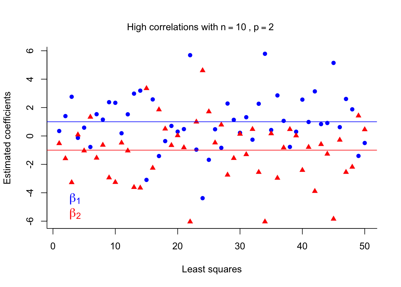

The figure plots the LS coefficients for 50 different sample sets. We can see that although the LS coefficients are unbiased estimates they are very unstable (high variance) in the presence of multicollinearity. This will affect the prediction error.

Issue due to \(p\) is close to \(n\)

Another issue is when \(p\) is close to \(n\). We investigate this case by running the simulation above again, but this time sampling both \(x_1\) and \(x_2\) from a standard normal distribution \(\mathcal{N}(0,1)\) (making the two predictors independent) and lowering the number of training points to 3. I have removed the detailed comments this time - try to see (and understand!) how it is different to the simulation above.

iter <- 50
n <- 3

b_LS <- matrix( NA, nrow = 2, ncol = iter )

for( i in 1:iter ){
  x1 <- rnorm( n )
  x2 <- rnorm( n )
  x <- cbind( x1, x2 )
  y <- x1 - x2 + rnorm( n )
  b_LS[,i]<- solve( t(x) %*% x ) %*% t(x) %*% y
}

plot( b_LS[1,], col = 'blue', pch = 16, ylim = c( min(b_LS), max(b_LS) ),
      ylab = 'Estimated coefficients', xlab = 'Least squares', bty ='l' )
points( b_LS[2,], col = 'red', pch = 17 )
abline( a = 1, b = 0, col = 'blue' ) 
abline( a = -1, b = 0, col='red' )

# Add a legend to this plot.
legend( 'bottomleft', cex = 1.3, text.col=c('blue','red'), 
        legend = c( expression( beta[1] ),expression( beta[2] ) ), bty = 'n' )

mtext( expression('No correlations with'~n == 3~','~ p == 2), 
       side = 3, line = -3, outer = TRUE )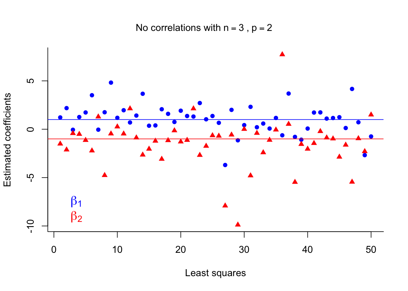

LS estimates suffer again from high variance. Of course, having only \(n=3\) training runs isn’t ideal in any situation, but it illustrates how LS estimates are affected when \(p\) is close to \(n\).

You may want to run the simulation above again but increase the number of training points and the number of predictors.

Many modern machine learning applications suffer from both of these problems we have just explored - that is, \(p\) can be large (and of similar magnitude to \(n\)) and it is very likely that there will be strong correlations among the many predictors!

To address these issues, one may adopt shrinkage methods. In previous lectures, we have seen discrete model search methods, where one option is to pick the best model based on information criteria (e.g. \(C_p,\) BIC, etc.). In this case, we generally seek the minimum of \[\underbrace{\mbox{model fit}}_{\mbox{RSS}}~ + ~{\mbox{penalty on model dimensionality}}\]
across models of differing dimensionality (number of predictors).

Shrinkage methods offer a continuous analogue (which is much faster). In this case we train only the full model, but the estimated regression coefficients minimise a general solution of the form \[\underbrace{\mbox{model fit}}_{\mbox{RSS}}~ + ~{\mbox{penalty on size of coefficients}}.\] This approach is called penalised or regularised regression.

6.2 Ridge Regression

Recall that Least Squares (LS) produces estimates of \(\beta_0,\, \beta_1,\, \beta_2,\, \ldots,\, \beta_p\) by minimising \[RSS = \sum_{i=1}^{n} \Bigg( y_i - \beta_0 - \sum_{j=1}^{p}\beta_j x_{ij}\Bigg)^2. \]

On the other hand, ridge regression minimises the cost function \[\underbrace{\sum_{i=1}^{n} \Bigg( y_i - \beta_0 - \sum_{j=1}^{p}\beta_j x_{ij}\Bigg)^2}_{\mbox{model fit}} + \underbrace{\lambda\sum_{j=1}^p\beta_j^2}_{\mbox{penalty}} = RSS + \lambda\sum_{j=1}^p\beta_j^2,\] where \(\lambda\ge 0\) is a tuning parameter. The role of this parameter is crucial; it controls the trade-off between model fit and the size of the coefficients.

In fact, the estimates based on the ridge regression cost function is the solution to the least squares problem subject to the constraint \(\sum_{j=1}^p\beta_j^2\leq c\) (Hint: Lagrange Multiplier). The following figure is the geometric interpretation of the ridge regression. 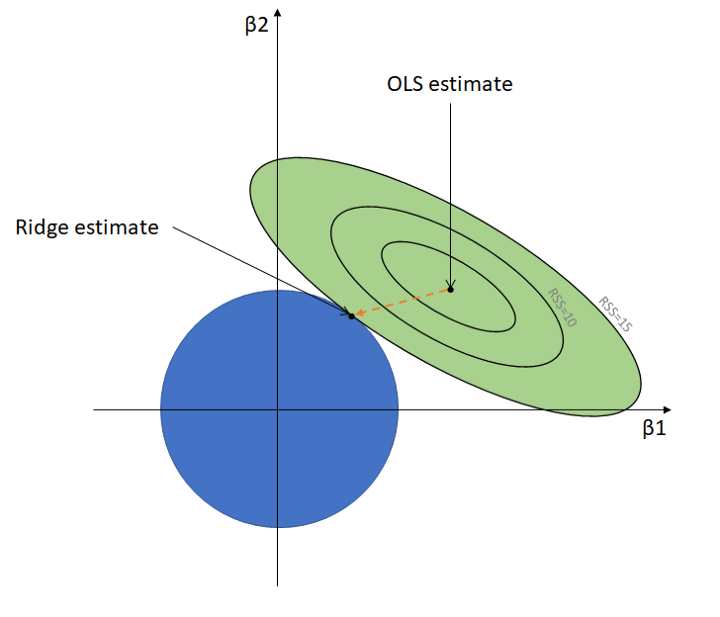The green contours represent the RSS in terms of different values of parameters of a linear regression model. Each contour is a connection of spots where the RSS is the same, centered with the (Ordinary) Least Squares estimate where the RSS is the lowest. Note that the LS estimate is the point where it best fits the training set (low-bias).

The blue circle represents the constraint \(\sum_{j=1}^p\beta_j^2\leq c\). Unlike the LS estimates, the ridge estimates change as the size of the blue circle changes. It is simply where the circle meets the most outer contour. How ridge regression works is how we tune the size of the circle, which is via tuning \(\lambda\).

From the ridge regression cost function, observe that:

• when \(\lambda=0\) the penalty term has no effect and the ridge solution is the same as the LS solution.
• as \(\lambda\) gets larger naturally the penalty term gets larger; so in order to minimise the entire function (model fit + penalty) the regression coefficients will necessarily get smaller!
• Unlike LS, ridge regression does not produce one set of coefficients, it produces different sets of coefficients for different values of \(\lambda\)!
• As \(\lambda\) is increasing the coefficients are shrunk towards 0 (for really large \(\lambda\) the coefficients are almost 0).

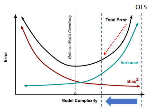
Tuning \(\lambda\) is in fact balancing the bias and variance.

Another way to view the ridge regression is via vector representation. That is the ridge estimates \(\hat{\boldsymbol{\beta}_R}=\left(\bf X^{\text{T}}\bf X +\lambda \boldsymbol{I}\right)^{-1} \bf X^{\text{T}}\bf Y\) shifts the \(\bf X^{\text{T}}\bf X\) in the LS estimates \(\hat{\boldsymbol{\beta}}=\left(\bf X^{\text{T}}\bf X \right)^{-1} \bf X^{\text{T}}\bf Y\) by \(\lambda \boldsymbol{I}\). Note in the cases of “perfect” multicollinearity and \(n<p\), \(\bf X^{\text{T}}\bf X\) is singular (non-invertible) and shifting \(\bf X^{\text{T}}\bf X\) by \(\lambda \boldsymbol{I}\) leads to an invertible matrix \(\left(\bf X^{\text{T}}\bf X +\lambda \boldsymbol{I}\right)\).

Demonstration in multicollinearity issue

The following code conducts the same simulation study as in the motivation and adds ridge estimates for comparison. Note that \((X^TX + \lambda I)^{-1}X^TY\) are the regression coefficient estimates for ridge regression.

# Number of iterations for the simulation study.
iter <- 50

# Number of training points.
n <- 10

# lambda coefficient - feel free to explore this parameter!
lambda <- 0.3

# Empty matrix of NAs for the regression coefficients, one for LS 
# and one for ridge.
b_LS <- matrix( NA, nrow = 2, ncol = iter )
b_ridge <- matrix( NA, nrow = 2, ncol = iter )

# For each iteration...
for( i in 1:iter ){

  # As we can see x2 is highly correlated with x1 - COLLINEARITY!
  x1 <- rnorm( n )
  x2 <- 0.9 * x1 + rnorm( n, 0, 0.2 )
  
  # Design matrix.
  x <- cbind( x1, x2 )
  
  # y = x1 - x2 + e, where error e is N(0,1)
  y <- x1 - x2 + rnorm( n )
  
  # LS regression components - the below calculation obtains them given the 
  # training data and response generated in this iteration, and stores 
  # those estimates in the relevant column of the matrix b_LS.
  b_LS[,i]<- solve( t(x) %*% x ) %*% t(x) %*% y
  
  # Ridge regression components - notice that the only difference relative 
  # to the LS estimates above is the addition of a lambda x identity matrix 
  # inside the inverse operator.
  b_ridge[,i]<- solve( t(x) %*% x + lambda * diag(2) ) %*% t(x) %*% y

}

# Now we plot the results.  First, split the plotting window 
# such that it has 1 row and 2 columns.
par(mfrow=c(1,2))

# Plot the LS estimates for beta_1.
plot( b_LS[1,], col = 'blue', pch = 16, ylim = c( min(b_LS), max(b_LS) ),
      ylab = 'Estimated coefficients', xlab = 'Least squares', bty ='l' )
# Add the LS estimates for beta_2 in a different colour.
points( b_LS[2,], col = 'red', pch = 17 )
# Add horizontal lines representing the true values of beta_1 and beta_2.
abline( a = 1, b = 0, col = 'blue' ) # Plot the true value of beta_1 = 1.
abline( a = -1, b = 0, col='red' ) # Plot the true value of beta_2 = -1.

# Do the same for the ridge estimates.
plot( b_ridge[1,], col = 'blue', pch = 16, ylim = c(min(b_LS), max(b_LS)), 
      ylab = 'Estimated coefficients', xlab = 'Ridge', bty ='l' )
points( b_ridge[2,], col = 'red', pch = 17 ) 
abline( a = 1, b = 0, col = 'blue' )
abline( a = -1, b = 0, col = 'red' )

# Add a legend to this plot.
legend( 'bottomleft', cex = 1.3, text.col=c('blue','red'), 
        legend = c( expression( beta[1] ),expression( beta[2] ) ), 
        bty = 'n' )

# Add a title over the top of both plots.
mtext( expression( 'High correlations with'~n == 10~','~ p == 2 ), 
       side = 3, line = -3, outer = TRUE )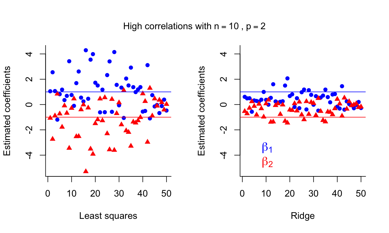

We can see that ridge regression introduces some bias but decreases the variance, which could result in better predictions.

Demonstration in \(p\) is close to \(n\) issue

Similarly, the following code conducts the same simulation study as in the motivation for \(p\) is close to \(n\) issue and adds ridge estimates for comparison.

iter <- 50
n <- 3
lambda <- 0.3

b_LS <- matrix( NA, nrow = 2, ncol = iter )
b_ridge <- matrix( NA, nrow = 2, ncol = iter )

for( i in 1:iter ){
  x1 <- rnorm( n )
  x2 <- rnorm( n )
  x <- cbind( x1, x2 )
  y <- x1 - x2 + rnorm( n )
  b_LS[,i]<- solve( t(x) %*% x ) %*% t(x) %*% y
  b_ridge[,i]<- solve( t(x) %*% x + lambda * diag(2) ) %*% t(x) %*% y
}

par(mfrow=c(1,2))
plot( b_LS[1,], col = 'blue', pch = 16, ylim = c( min(b_LS), max(b_LS) ),
      ylab = 'Estimated coefficients', xlab = 'Least squares', bty ='l' )
points( b_LS[2,], col = 'red', pch = 17 )
abline( a = 1, b = 0, col = 'blue' ) 
abline( a = -1, b = 0, col='red' )

plot( b_ridge[1,], col = 'blue', pch = 16, ylim = c(min(b_LS), max(b_LS)), 
      ylab = 'Estimated coefficients', xlab = 'Ridge', bty ='l' )
points( b_ridge[2,], col = 'red', pch = 17 ) 
abline( a = 1, b = 0, col = 'blue' )
abline( a = -1, b = 0, col = 'red' )

# Add a legend to this plot.
legend( 'bottomleft', cex = 1.3, text.col=c('blue','red'), 
        legend = c( expression( beta[1] ),expression( beta[2] ) ), bty = 'n' )

mtext( expression('No correlations with'~n == 3~','~ p == 2), 
       side = 3, line = -3, outer = TRUE )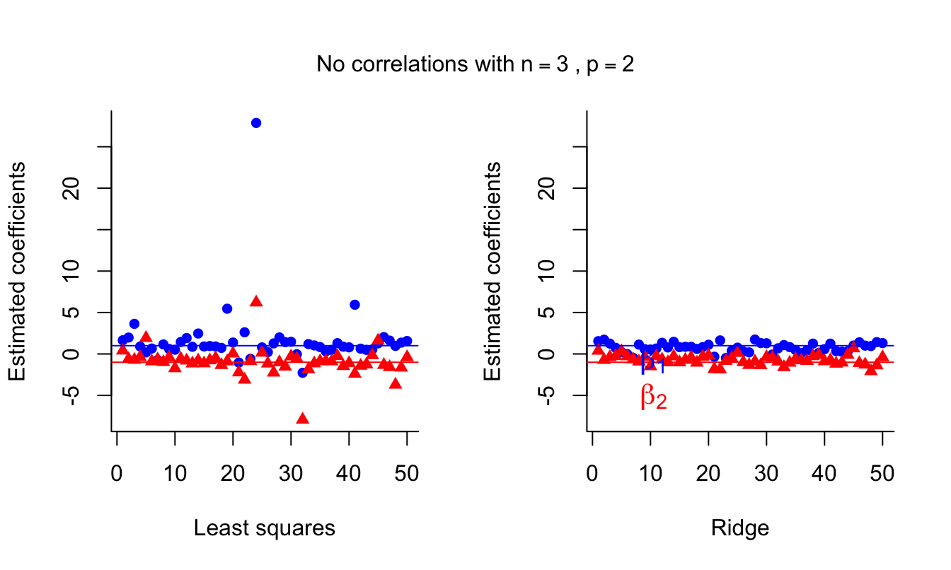

Ridge estimates are again more stable and can be an improvement over LS.

Scalability and Feature Selection

• Ridge regression is applicable for any number of predictors even when \(n < p\), remember that LS solutions do not exist in this case. It is also much faster than the model-search based methods since we train only one model.
• Strictly speaking, ridge regression does not perform feature selection (since the coefficients are almost never exactly 0), but it can give us a good idea of which predictors are not influential and can be combined with post-hoc analysis based on ranking the absolute values of the coefficients.

Scaling

• The LS estimates are scale invariant: multiplying a feature \(X_j\) by some constant \(c\) will scale down \(\hat{\beta}_j\) by \(1/c\), so \(X_j\hat{\beta}_j\) will remain unaffected.
• In ridge regression (and any shrinkage method) the scaling of the features matters! If a relevant feature is in a smaller scale (that is, the numbers are smaller, e.g. if you use metres as opposed to millimetres) in relation to other features it will have a larger coefficient which constitutes a greater proportion of the penalty term and will thus shrink proportionally faster to zero.
• So, we want the features to be on the same scale.
• In practice, we standardise: \[ \tilde{x}_{ij} = \frac{x_{ij}}{\sqrt{\sum\frac{1}{n} (x_{ij}-\bar{x}_j)^2}},\] so that all predictors have variance equal to one.

Practical Demonstration

We will continue analysing the Hitters dataset included in package ISLR, this time applying the method of ridge regression.

We perform the usual steps of removing missing data, as seen in Section 5.4.

library(ISLR)
Hitters = na.omit(Hitters)
dim(Hitters)

## [1] 263  20

sum(is.na(Hitters))

## [1] 0

To conduct ridge regression, the first thing to do is to load up the package glmnet (remember to run the command install.packages('glmnet') the first time).

library(glmnet)

## Loading required package: Matrix

## Loaded glmnet 4.1-4

Initially, we will make use of function glmnet() which implements ridge regression without cross-validation, but it does give a range of solutions over a grid of \(\lambda\) values. The grid is produced automatically - we do not need to specify anything. Of course, if we want to we can define the grid manually. Let’s have a look first at the help document of glmnet().

?glmnet

A first important thing to observe is that glmnet() requires a different syntax than regsubsets() for declaring the response variable and the predictors. Now the response should be a vector and the predictor variables must be stacked column-wise as a matrix. This is easy to do for the response. For the predictors we have to make use of the model.matrix() command. Let us define as y the response and as x the matrix of predictors.

y = Hitters$Salary
x = model.matrix(Salary~., Hitters)[,-1] # Here we exclude the first column 
                                         # because it corresponds to the 
                                         # intercept.
head(x)

##                   AtBat Hits HmRun Runs RBI Walks Years CAtBat CHits CHmRun
## -Alan Ashby         315   81     7   24  38    39    14   3449   835     69
## -Alvin Davis        479  130    18   66  72    76     3   1624   457     63
## -Andre Dawson       496  141    20   65  78    37    11   5628  1575    225
## -Andres Galarraga   321   87    10   39  42    30     2    396   101     12
## -Alfredo Griffin    594  169     4   74  51    35    11   4408  1133     19
## -Al Newman          185   37     1   23   8    21     2    214    42      1
##                   CRuns CRBI CWalks LeagueN DivisionW PutOuts Assists Errors
## -Alan Ashby         321  414    375       1         1     632      43     10
## -Alvin Davis        224  266    263       0         1     880      82     14
## -Andre Dawson       828  838    354       1         0     200      11      3
## -Andres Galarraga    48   46     33       1         0     805      40      4
## -Alfredo Griffin    501  336    194       0         1     282     421     25
## -Al Newman           30    9     24       1         0      76     127      7
##                   NewLeagueN
## -Alan Ashby                1
## -Alvin Davis               0
## -Andre Dawson              1
## -Andres Galarraga          1
## -Alfredo Griffin           0
## -Al Newman                 0

See how the command model.matrix() automatically transformed the categorical variables in Hitters with names League, Division and NewLeague to dummy variables with names LeagueN, DivisionW and NewLeagueN. Other important things that we see in the help document are that glmnet() uses a grid of 100 values for \(\lambda\) (nlambda = 100) and that parameter alpha is used to select between ridge implementation and lasso implementation. The default option is alpha = 1 which runs lasso (see Chapter 6.3) - for ridge we have to set alpha = 0. Finally we see the default option standardize = TRUE, which means we do not need to standardize the predictor variables manually.

Now we are ready to run our first ridge regression!

ridge = glmnet(x, y, alpha = 0)

Using the command names() we can find what is returned by the function. The most important components are "beta" and "lambda". We can easily extract each using the $ symbol.

names(ridge)

##  [1] "a0"        "beta"      "df"        "dim"       "lambda"    "dev.ratio"
##  [7] "nulldev"   "npasses"   "jerr"      "offset"    "call"      "nobs"

ridge$lambda

##   [1] 255282.09651 232603.53864 211939.68135 193111.54419 175956.04684
##   [6] 160324.59659 146081.80131 133104.29670 121279.67783 110505.52551
##  [11] 100688.51919  91743.62866  83593.37754  76167.17227  69400.69061
##  [16]  63235.32454  57617.67259  52499.07736  47835.20402  43585.65633
##  [21]  39713.62675  36185.57761  32970.95062  30041.90224  27373.06245
##  [26]  24941.31502  22725.59734  20706.71790  18867.19015  17191.08098
##  [31]  15663.87273  14272.33745  13004.42232  11849.14529  10796.49988
##  [36]   9837.36858   8963.44387   8167.15622   7441.60857   6780.51658
##  [41]   6178.15417   5629.30398   5129.21213   4673.54706   4258.36202
##  [46]   3880.06088   3535.36696   3221.29471   2935.12376   2674.37546
##  [51]   2436.79131   2220.31349   2023.06696   1843.34326   1679.58573
##  [56]   1530.37596   1394.42158   1270.54501   1157.67329   1054.82879
##  [61]    961.12071    875.73739    797.93930    727.05257    662.46322
##  [66]    603.61181    549.98860    501.12913    456.61020    416.04621
##  [71]    379.08581    345.40887    314.72370    286.76451    261.28915
##  [76]    238.07694    216.92684    197.65566    180.09647    164.09720
##  [81]    149.51926    136.23638    124.13351    113.10583    103.05782
##  [86]     93.90245     85.56042     77.95946     71.03376     64.72332
##  [91]     58.97348     53.73443     48.96082     44.61127     40.64813
##  [96]     37.03706     33.74679     30.74882     28.01718     25.52821

dim(ridge$beta)

## [1]  19 100

ridge$beta[,1:3]

## 19 x 3 sparse Matrix of class "dgCMatrix"
##                                                         s0            s1
## AtBat       0.00000000000000000000000000000000000122117189  0.0023084432
## Hits        0.00000000000000000000000000000000000442973647  0.0083864077
## HmRun       0.00000000000000000000000000000000001784943997  0.0336900933
## Runs        0.00000000000000000000000000000000000749101852  0.0141728323
## RBI         0.00000000000000000000000000000000000791287003  0.0149583386
## Walks       0.00000000000000000000000000000000000931296087  0.0176281785
## Years       0.00000000000000000000000000000000003808597789  0.0718368521
## CAtBat      0.00000000000000000000000000000000000010484944  0.0001980310
## CHits       0.00000000000000000000000000000000000038587587  0.0007292122
## CHmRun      0.00000000000000000000000000000000000291003649  0.0054982153
## CRuns       0.00000000000000000000000000000000000077415313  0.0014629668
## CRBI        0.00000000000000000000000000000000000079894300  0.0015098418
## CWalks      0.00000000000000000000000000000000000084527517  0.0015957724
## LeagueN    -0.00000000000000000000000000000000001301216845 -0.0230232091
## DivisionW  -0.00000000000000000000000000000000017514595071 -0.3339842326
## PutOuts     0.00000000000000000000000000000000000048911970  0.0009299203
## Assists     0.00000000000000000000000000000000000007989093  0.0001517222
## Errors     -0.00000000000000000000000000000000000037250274 -0.0007293365
## NewLeagueN -0.00000000000000000000000000000000000258502617 -0.0036169801
##                       s2
## AtBat       0.0025301407
## Hits        0.0091931957
## HmRun       0.0369201974
## Runs        0.0155353349
## RBI         0.0163950163
## Walks       0.0193237654
## Years       0.0787191800
## CAtBat      0.0002170325
## CHits       0.0007992257
## CHmRun      0.0060260057
## CRuns       0.0016034328
## CRBI        0.0016548119
## CWalks      0.0017488195
## LeagueN    -0.0250669217
## DivisionW  -0.3663713386
## PutOuts     0.0010198028
## Assists     0.0001663687
## Errors     -0.0008021006
## NewLeagueN -0.0038293583

As we see above glmnet() defines the grid starting with large values of \(\lambda\). This is because this helps speed up the optimisation procedure. Also, glmnet() performs some internal checks on the predictor variables in order to define the grid values. Therefore, it is generally better to let glmnet() define the grid automatically, rather than manually defining a grid. We further see that as expected ridge$beta had 19 rows (number of predictors) and 100 columns (length of the grid). Above the first 3 columns are displayed. Notice that ridge$beta does not return the estimates of the intercepts. We can use the command coef() for this, which returns all betas.

coef(ridge)[,1:3]

## 20 x 3 sparse Matrix of class "dgCMatrix"
##                                                           s0             s1
## (Intercept) 535.92588212927762469917070120573043823242187500 527.9266102513
## AtBat         0.00000000000000000000000000000000000122117189   0.0023084432
## Hits          0.00000000000000000000000000000000000442973647   0.0083864077
## HmRun         0.00000000000000000000000000000000001784943997   0.0336900933
## Runs          0.00000000000000000000000000000000000749101852   0.0141728323
## RBI           0.00000000000000000000000000000000000791287003   0.0149583386
## Walks         0.00000000000000000000000000000000000931296087   0.0176281785
## Years         0.00000000000000000000000000000000003808597789   0.0718368521
## CAtBat        0.00000000000000000000000000000000000010484944   0.0001980310
## CHits         0.00000000000000000000000000000000000038587587   0.0007292122
## CHmRun        0.00000000000000000000000000000000000291003649   0.0054982153
## CRuns         0.00000000000000000000000000000000000077415313   0.0014629668
## CRBI          0.00000000000000000000000000000000000079894300   0.0015098418
## CWalks        0.00000000000000000000000000000000000084527517   0.0015957724
## LeagueN      -0.00000000000000000000000000000000001301216845  -0.0230232091
## DivisionW    -0.00000000000000000000000000000000017514595071  -0.3339842326
## PutOuts       0.00000000000000000000000000000000000048911970   0.0009299203
## Assists       0.00000000000000000000000000000000000007989093   0.0001517222
## Errors       -0.00000000000000000000000000000000000037250274  -0.0007293365
## NewLeagueN   -0.00000000000000000000000000000000000258502617  -0.0036169801
##                         s2
## (Intercept) 527.1582433004
## AtBat         0.0025301407
## Hits          0.0091931957
## HmRun         0.0369201974
## Runs          0.0155353349
## RBI           0.0163950163
## Walks         0.0193237654
## Years         0.0787191800
## CAtBat        0.0002170325
## CHits         0.0007992257
## CHmRun        0.0060260057
## CRuns         0.0016034328
## CRBI          0.0016548119
## CWalks        0.0017488195
## LeagueN      -0.0250669217
## DivisionW    -0.3663713386
## PutOuts       0.0010198028
## Assists       0.0001663687
## Errors       -0.0008021006
## NewLeagueN   -0.0038293583

We can produce a plot similar to the ones seen previously via the following simple code. On the left we have the regularisation paths based on \(\log\lambda\). Specifying xvar is important, as the default is to plot the \(\ell_1\)-norm on the \(x\)-axis (see Chapter 6.3). Don’t worry about the row of 19’s along the top of the plot for now, except to note that this is the number of predictor variables. The reason for their presence will become clear in Chapter 6.3.

plot(ridge, xvar = 'lambda')

6.3 Lasso Regression

Disadvantage of Ridge Regression

• Unlike model search methods which select models that include subsets of predictors, ridge regression will include all \(p\) predictors.
• Even for those predictors that are irrelevant to the response, their coefficients will only get close to zero but never exactly zero!
• Even if we could perform a post-hoc analysis to reduce the number of predictors, ideally we would like a method that sets these coefficients equal to zero automatically.

The Lasso

Similar to ridge regression it penalises the size of the coefficients, but instead of the squares it penalises the absolute values. The lasso regression estimates minimise the quantity \[{\sum_{i=1}^{n} \Bigg( y_i - \beta_0 - \sum_{j=1}^{p}\beta_j x_{ij}\Bigg)^2} + {\lambda\sum_{j=1}^p|\beta_j|} = RSS + \lambda\sum_{j=1}^p|\beta_j|\]

The only difference is that the \(\beta_j^2\) term in the ridge regression penalty has been replaced by \(|\beta_j|\) in the lasso penalty.

Lasso offers the same benefits as ridge:

• it introduces some bias but decreases the variance, so it improves predictive performance.
• it is extremely scalable and can cope with \(n<p\) problems.

As with ridge regression, the lasso shrinks the coefficient estimates towards zero. However, in the case of the lasso, the \(\ell_1\) penalty has the effect of forcing some of the coefficient estimates to be exactly equal to zero when the tuning parameter \(\lambda\) is sufficiently large. Hence, much like best subset selection, the lasso performs variable selection. As a result, models generated from the lasso are generally much easier to interpret than those produced by ridge regression. We say that the lasso yields sparse models, that is, models that involve only a subset of the variables. As with ridge regression, the choice of \(\lambda\) is critical, but we defer discussion of this until Chapter 6.4.

Ridge vs. Lasso

Here we make some comparisons between ridge regression and lasso regression.

Ridge and Lasso with \(\ell\)-norms

We have talked a little bit about the \(\ell\)-norms, but here we clarify the difference between ridge and lasso using them.

Lets just denote \(\beta=(\beta_1,\ldots,\beta_p)\). Then a more compact representation of ridge and lasso minimisation is the following:

• Ridge: \({\sum_{i=1}^{n} \Bigg( y_i - \beta_0 - \sum_{j=1}^{p}\beta_j x_{ij}\Bigg)^2} + {\lambda\Vert\beta\Vert_2^2}\), where \(\Vert\beta\Vert_2=\sqrt{\beta_1^2 + \ldots + \beta_p^2}\) is the \(\ell_2\)-norm of \(\beta\).
• Lasso: \({\sum_{i=1}^{n} \Bigg( y_i - \beta_0 - \sum_{j=1}^{p}\beta_j x_{ij}\Bigg)^2} + {\lambda\Vert\beta\Vert_1}\), where \(\Vert\beta\Vert_1={|\beta_1| + \ldots + |\beta_p|}\) is the \(\ell_1\)-norm of \(\beta\).

That is why we say that ridge uses \(\ell_2\)-penalisation, while lasso uses \(\ell_1\)-penalisation.

Ridge and Lasso as Constrained Optimisation Problems

• Ridge: minimise \(\sum_{i=1}^{n} \Bigg( y_i - \beta_0 - \sum_{j=1}^{p}\beta_j x_{ij}\Bigg)^2\) subject to \(\sum_{j=1}^p\beta_j^2 \le c\).
• Lasso: minimise \(\sum_{i=1}^{n} \Bigg( y_i - \beta_0 - \sum_{j=1}^{p}\beta_j x_{ij}\Bigg)^2\) subject to \(\sum_{j=1}^p|\beta_j| \le c\).
• The words subject to above essentially imposes the corresponding constraints.
• Threshold \(c\) may be considered as a budget: large \(c\) allows coefficients to be large.
• There is a one-to-one correspondence between penalty parameter \(\lambda\) and threshold \(c\), meaning for any given regression problem, given a specific \(\lambda\) there always exists a corresponding \(c\), and vice-versa.
• When \(\lambda\) is large, then \(c\) is small, and vice-versa!
• The ridge constraint is smooth, while the lasso constraint is edgy. This is nicely illustrated in Figure 6.1. \(\beta_1\) and \(\beta_2\) are not allowed to go outside of the red areas.

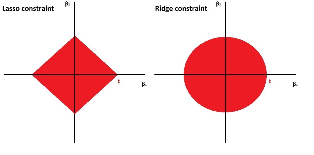
Figure 6.1: Left: the constraint \(|\beta_1| + |\beta_2| \leq c\), Right: the constraint \(\beta_1^2 + \beta_2^2 \leq c\).

It is this difference between the smooth and edgy constraints that result in the lasso having coefficient estimates that are exactly zero and ridge not. We illustrate this even further in Figure 6.2. The least squares solution is marked as \(\hat{\beta}\), while the blue diamond and circle represent the lasso and ridge regression constraints (as in Figure 6.1). If \(c\) is sufficiently large (making \(c\) larger results in the diamond and circle respectively getting larger), then the constraint regions will contain \(\hat{\beta}\), and so the ridge and lasso estimates will be the same as the least squares estimates.

The contours that are centered around \(\hat{\beta}\) represent regions of constant RSS. As the ellipses expand away from the least squares coefficient estimates, the RSS increases. The lasso and ridge regression coefficient estimates are given by the first point at which an ellipse contacts the constraint region.

Figure 6.2: Contours of the error and constraint functions for the lasso (left) and ridge regression (right). The solid blue areas are the constraint regions \(|\beta_1| + |\beta_2| \leq c\) and \(\beta_1^2 + \beta_2^2 \leq c\) respectively. The red ellipses are the contours of the Residual Sum of Squares, with the values along each contour being the same, and outer contours having a higher value (least squares \(\hat{\beta}\) has minimal RSS).

Since ridge regression has a circular constraint with no sharp points, this intersection will generally NOT occur on an axis, and so the ridge regression coefficient estimates will be exclusively non-zero. However, the lasso constraint has corners at each of the axes, and so the ellipse will often intersect the constraint region at an axis (in fact in the higher dimensional case, the chance of the hyper-ellipse hitting the corners of the hyper-dimond gets much higher). When this occurs, one of the coefficient estimates will equal zero. In Figure 6.2, the intersection occurs at \(\beta_1=0\), and so the resulting model will only include \(\beta_2\).

Different \(\lambda\)’s

• Both ridge and lasso are convex optimisation problems Boyd and Vandenberghe (2009).
• In optimisation, convexity is a desired property.
• In fact, the ridge solution exists in closed form (meaning we have a formula for it).
• Lasso does not have a closed form solution, but nowadays there exist very efficient optimisation algorithms for the lasso solution.
• Package glmnet in R implements coordinate descent (very fast) – same time to solve ridge and lasso.
• Due to clever optimisation tricks, finding the solutions for multiple \(\lambda\)’s takes the same time as finding the solution for one single \(\lambda\) value. This is very useful: it implies that we can obtain the solutions for a grid of values of \(\lambda\) very fast and then pick a specific \(\lambda\) that is optimal in regard to some objective function (see Chapter 6.4).

Predictive Performance

So, lasso has a clear advantage over ridge - it can set coefficients equal to zero!

This must mean that it is also better for prediction, right? Well, not necessarily. Things are a bit more complicated than that\(...\)it all comes down to the nature of the actual underlying mechanism. Let’s explain this rather cryptic answer\(...\)

Generally…

• When the actual data-generating mechanism is sparse lasso has the advantage.
• When the actual data-generating mechanism is dense ridge has the advantage.

Sparse mechanisms: Few predictors are relevant to the response \(\rightarrow\) good setting for lasso regression.

Dense mechanisms: A lot of predictors are relevant to the response \(\rightarrow\) good setting for ridge regression.

Figure 6.3 roughly illustrates how prediction mean square error may depend on the density of the mechanism (number of predictors).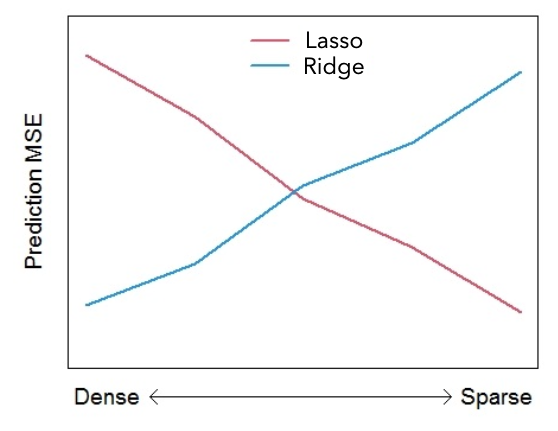

Figure 6.3: Rough illustration of the effect of mechanism density on prediction Mean Squared Error.

This figure really is a rough extreme illustration! The actual performance will also depend upon:

• Signal strength (the magnitude of the effects of the relevant variables).
• The correlation structure among predictors.
• Sample size \(n\) vs. number of predictors \(p\).

So…which is better?

• In general, none of the two shrinkage methods will dominate in terms of predictive performance under all settings.
• Lasso performs better when few predictors have a substantial effect on the response variable.
• Ridge performs better when a lot of predictors have a substantial effect on the response.
• Keep in mind: a few and a lot are always relative to the total number of available predictors.
• Overall: in most applications, lasso is more robust.

Question: What should I do if I have to choose between ridge and lasso?

Answer: Keep a part of the data for testing purposes only and compare the predictive performance of the two methods.

Practical Demonstration

We will continue analysing the Hitters dataset included in package ISLR, this time applying lasso regression.

We perform the usual steps of removing missing data as we have seen in previous practical demonstrations.

library(ISLR)
Hitters = na.omit(Hitters)
dim(Hitters)

## [1] 263  20

sum(is.na(Hitters))

## [1] 0

We will now use glmnet() to implement lasso regression.

library(glmnet)

Having learned how to implement ridge regression in previous section the analysis is very easy. To run lasso all we have to do is remove the option alpha = 0. We do not need to specify explicitly alpha = 1 because this is the default option in glmnet().

In this part again we call the response y and extract the matrix of predictors, which we call x using the command model.matrix().

y = Hitters$Salary
x = model.matrix(Salary~., Hitters)[,-1] # Here we exclude the first column 
                                         # because it corresponds to the 
                                         # intercept.
head(x)

##                   AtBat Hits HmRun Runs RBI Walks Years CAtBat CHits CHmRun
## -Alan Ashby         315   81     7   24  38    39    14   3449   835     69
## -Alvin Davis        479  130    18   66  72    76     3   1624   457     63
## -Andre Dawson       496  141    20   65  78    37    11   5628  1575    225
## -Andres Galarraga   321   87    10   39  42    30     2    396   101     12
## -Alfredo Griffin    594  169     4   74  51    35    11   4408  1133     19
## -Al Newman          185   37     1   23   8    21     2    214    42      1
##                   CRuns CRBI CWalks LeagueN DivisionW PutOuts Assists Errors
## -Alan Ashby         321  414    375       1         1     632      43     10
## -Alvin Davis        224  266    263       0         1     880      82     14
## -Andre Dawson       828  838    354       1         0     200      11      3
## -Andres Galarraga    48   46     33       1         0     805      40      4
## -Alfredo Griffin    501  336    194       0         1     282     421     25
## -Al Newman           30    9     24       1         0      76     127      7
##                   NewLeagueN
## -Alan Ashby                1
## -Alvin Davis               0
## -Andre Dawson              1
## -Andres Galarraga          1
## -Alfredo Griffin           0
## -Al Newman                 0

We then run lasso regression.

lasso = glmnet(x, y)

lambda and beta are still the most important components of the output.

names(lasso)

##  [1] "a0"        "beta"      "df"        "dim"       "lambda"    "dev.ratio"
##  [7] "nulldev"   "npasses"   "jerr"      "offset"    "call"      "nobs"

lasso$lambda

##  [1] 255.2820965 232.6035386 211.9396813 193.1115442 175.9560468 160.3245966
##  [7] 146.0818013 133.1042967 121.2796778 110.5055255 100.6885192  91.7436287
## [13]  83.5933775  76.1671723  69.4006906  63.2353245  57.6176726  52.4990774
## [19]  47.8352040  43.5856563  39.7136268  36.1855776  32.9709506  30.0419022
## [25]  27.3730624  24.9413150  22.7255973  20.7067179  18.8671902  17.1910810
## [31]  15.6638727  14.2723374  13.0044223  11.8491453  10.7964999   9.8373686
## [37]   8.9634439   8.1671562   7.4416086   6.7805166   6.1781542   5.6293040
## [43]   5.1292121   4.6735471   4.2583620   3.8800609   3.5353670   3.2212947
## [49]   2.9351238   2.6743755   2.4367913   2.2203135   2.0230670   1.8433433
## [55]   1.6795857   1.5303760   1.3944216   1.2705450   1.1576733   1.0548288
## [61]   0.9611207   0.8757374   0.7979393   0.7270526   0.6624632   0.6036118
## [67]   0.5499886   0.5011291   0.4566102   0.4160462   0.3790858   0.3454089
## [73]   0.3147237   0.2867645   0.2612891   0.2380769   0.2169268   0.1976557
## [79]   0.1800965   0.1640972

dim(lasso$beta)

## [1] 19 80

lasso$beta[,1:3]   # this returns only the predictor coefficients

## 19 x 3 sparse Matrix of class "dgCMatrix"
##            s0         s1         s2
## AtBat       . .          .         
## Hits        . .          .         
## HmRun       . .          .         
## Runs        . .          .         
## RBI         . .          .         
## Walks       . .          .         
## Years       . .          .         
## CAtBat      . .          .         
## CHits       . .          .         
## CHmRun      . .          .         
## CRuns       . .          0.01515244
## CRBI        . 0.07026614 0.11961370
## CWalks      . .          .         
## LeagueN     . .          .         
## DivisionW   . .          .         
## PutOuts     . .          .         
## Assists     . .          .         
## Errors      . .          .         
## NewLeagueN  . .          .

coef(lasso)[,1:3]  # this returns intercept + predictor coefficients

## 20 x 3 sparse Matrix of class "dgCMatrix"
##                   s0           s1           s2
## (Intercept) 535.9259 512.70866859 490.92996088
## AtBat         .        .            .         
## Hits          .        .            .         
## HmRun         .        .            .         
## Runs          .        .            .         
## RBI           .        .            .         
## Walks         .        .            .         
## Years         .        .            .         
## CAtBat        .        .            .         
## CHits         .        .            .         
## CHmRun        .        .            .         
## CRuns         .        .            0.01515244
## CRBI          .        0.07026614   0.11961370
## CWalks        .        .            .         
## LeagueN       .        .            .         
## DivisionW     .        .            .         
## PutOuts       .        .            .         
## Assists       .        .            .         
## Errors        .        .            .         
## NewLeagueN    .        .            .

We see that lasso$beta has 19 rows (number of predictors) and 80 columns. (Note the number of \(\lambda\) is less than the default setting, 100 (The reason lies in the stopping criteria of the algorithm. According to the default internal settings, the computations stop if either the fractional change in deviance (relates to the log-likelihoods) down the path is less than \(10^5\) or the fraction of explained deviance (similar to the concept of \(R^2\)) reaches 0.999). Using coef instead includes the intercept term. The key difference this time (in comparison to the application to ridge regression is that some of the elements of the output are replaced with a “.”, indicating that the corresponding predictor is not included in the lasso regression model with that value of \(\lambda\).

We now produce a plot of regularisation (Regularisation refers to the technique that discourages learning a more complex or flexible model, so as to avoid the risk of overfitting.) paths based on \(\log\lambda\). The numbers along the top now correspond to the number of predictors in the model for the corresponding (log) \(\lambda\) values. Recall the row of 19’s across the top of the corresponding plot for ridge regression - this is because for ridge we always include all predictors.

plot(lasso, xvar = 'lambda')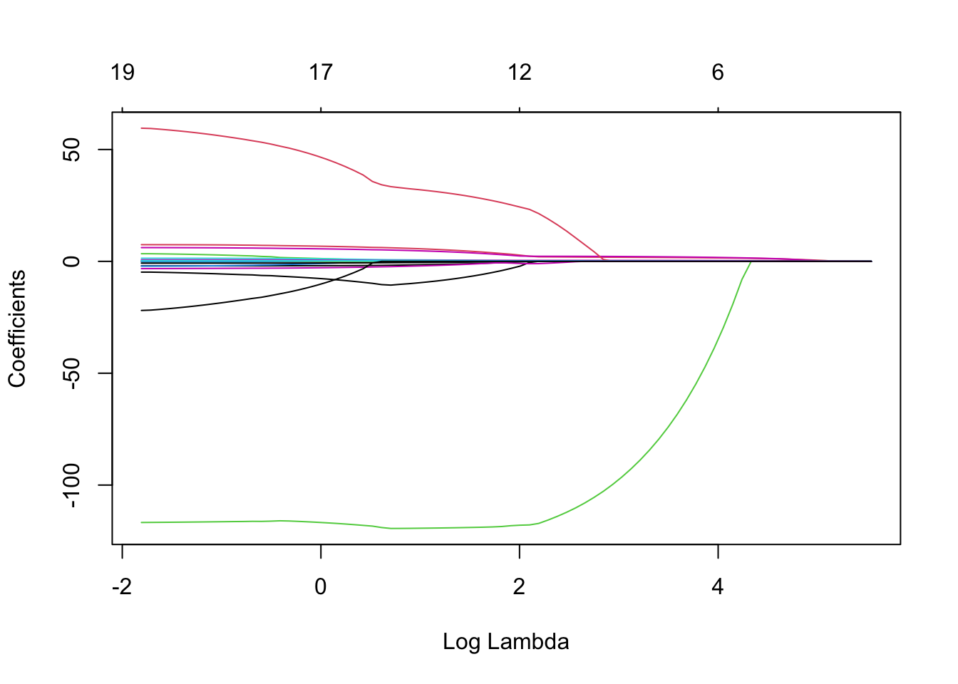

6.4 Choosing \(\lambda\)

Importance of \(\lambda\)

• As we have seen, the penalty parameter \(\lambda\) is of crucial importance in penalised regression.
• For \(\lambda=0\) we essentially just get the LS estimates of the full model.
• For very large \(\lambda\): all ridge estimates become extremely small, while all lasso estimates are exactly zero!

We require a principled way to fine-tune \(\lambda\) in order to get optimal results.

Selection Criteria?

• In Chapter 4.6, we used the selection criteria \(C_p\), BIC and adjusted-\(R^2\) as criteria for choosing particular models during model search methods.
• Perhaps we can do that here, for instance, by defining a grid of values for \(\lambda\) and calculating the corresponding \(C_p\) under each model, before then finding the model with the corresponding \(\lambda\) that yields the lowest \(C_p\) value?
• Not really - the problem is that all these techniques depend on model dimensionality (number of predictors).
• With model-search methods we choose a model with \(d\) predictors, so it is clear that the model’s dimensionality is \(d\).
• Shrinkage methods, however, penalise dimensionality in a different way - the very notion of model dimensionality becomes obscure somehow - does a constrained predictor count towards dimensionality in the same way as an unconstrained one?

Cross-Validation

The only viable strategy is \(K\)-fold cross-validation. The steps are the following:

1. Choose the number of folds \(K\).
2. Split the data accordingly into training and testing sets.
3. Define a grid of values for \(\lambda\).
4. For each \(\lambda\) calculate the validation Mean Squared Error (MSE) within each fold.
5. For each \(\lambda\) calculate the overall cross-validation MSE.
6. Locate under which \(\lambda\) cross-validation MSE is minimised. This value of \(\lambda\) is known as the minimum_CV \(\lambda\).

Seems difficult, but fortunately glmnet in R will do all of these things for us automatically! We will explore using cross-validation for choosing \(\lambda\) further via practical demonstration.

Practical Demonstration

We will continue analysing the Hitters dataset included in package ISLR.

Perform the usual steps of removing missing data.

library(ISLR)
Hitters = na.omit(Hitters)
dim(Hitters)

## [1] 263  20

sum(is.na(Hitters))

## [1] 0

Ridge regression

In this part again we call the response y and extract the matrix of predictors, which we call x using the command model.matrix().

y = Hitters$Salary
x = model.matrix(Salary~., Hitters)[,-1] # Here we exclude the first column 
                                         # because it corresponds to the 
                                         # intercept term.
head(x)

##                   AtBat Hits HmRun Runs RBI Walks Years CAtBat CHits CHmRun
## -Alan Ashby         315   81     7   24  38    39    14   3449   835     69
## -Alvin Davis        479  130    18   66  72    76     3   1624   457     63
## -Andre Dawson       496  141    20   65  78    37    11   5628  1575    225
## -Andres Galarraga   321   87    10   39  42    30     2    396   101     12
## -Alfredo Griffin    594  169     4   74  51    35    11   4408  1133     19
## -Al Newman          185   37     1   23   8    21     2    214    42      1
##                   CRuns CRBI CWalks LeagueN DivisionW PutOuts Assists Errors
## -Alan Ashby         321  414    375       1         1     632      43     10
## -Alvin Davis        224  266    263       0         1     880      82     14
## -Andre Dawson       828  838    354       1         0     200      11      3
## -Andres Galarraga    48   46     33       1         0     805      40      4
## -Alfredo Griffin    501  336    194       0         1     282     421     25
## -Al Newman           30    9     24       1         0      76     127      7
##                   NewLeagueN
## -Alan Ashby                1
## -Alvin Davis               0
## -Andre Dawson              1
## -Andres Galarraga          1
## -Alfredo Griffin           0
## -Al Newman                 0

For implementing cross-validation (CV) in order to select \(\lambda\) we will have to use the function cv.glmnet() from library glmnet. After loading library glmnet, we have a look at the help document by typing ?cv.glmnet. We see the argument nfolds = 10, so the default option is 10-fold CV (this is something we can change if we want to).

To perform cross-validation for selection of \(\lambda\) we simply run the following:

library(glmnet)

set.seed(1)
ridge.cv = cv.glmnet(x, y, alpha=0)

We extract the names of the output components as follows:

names( ridge.cv )

##  [1] "lambda"     "cvm"        "cvsd"       "cvup"       "cvlo"      
##  [6] "nzero"      "call"       "name"       "glmnet.fit" "lambda.min"
## [11] "lambda.1se" "index"

lambda.min provides the optimal value of \(\lambda\) as suggested by the cross-validation MSEs.

ridge.cv$lambda.min

## [1] 25.52821

lambda.1se provides a different value of \(\lambda\), known as the 1-standard error (1-se) \(\lambda\). This is the maximum value that \(\lambda\) can take while still falling within the one standard error interval of the minimum_CV \(\lambda\).

ridge.cv$lambda.1se 

## [1] 1843.343

We see that in this case the 1-se \(\lambda\) is much larger than the min-CV \(\lambda\). This means that we expect the coefficients under 1-se \(\lambda\) to be much smaller. We can see that this is indeed the case by looking at the corresponding coefficients from the two models, rounding them to 3 decimal places.

round(cbind(
  coef(ridge.cv, s = 'lambda.min'),
  coef(ridge.cv, s = 'lambda.1se')),  
  digits = 3 )

## 20 x 2 sparse Matrix of class "dgCMatrix"
##                   s1      s1
## (Intercept)   81.127 159.797
## AtBat         -0.682   0.102
## Hits           2.772   0.447
## HmRun         -1.366   1.289
## Runs           1.015   0.703
## RBI            0.713   0.687
## Walks          3.379   0.926
## Years         -9.067   2.715
## CAtBat        -0.001   0.009
## CHits          0.136   0.034
## CHmRun         0.698   0.254
## CRuns          0.296   0.069
## CRBI           0.257   0.071
## CWalks        -0.279   0.066
## LeagueN       53.213   5.396
## DivisionW   -122.834 -29.097
## PutOuts        0.264   0.068
## Assists        0.170   0.009
## Errors        -3.686  -0.236
## NewLeagueN   -18.105   4.458

Let’s plot the results based on the output of ridge.cv using plot. What is plotted is the estimated CV MSE for each value of (log) \(\lambda\) on the \(x\)-axis. The dotted line on the far left indicates the value of \(\lambda\) which minimises CV error. The dotted line roughly in the middle of the \(x\)-axis indicates the 1-standard-error \(\lambda\) - recall that this is the maximum value that \(\lambda\) can take while still falling within the on standard error interval of the minimum-CV \(\lambda\). The second line of code has manually added a dot-dash horizontal line at the upper end of the 1-standard deviation interval of the MSE at the minimum-CV \(\lambda\) to illustrate this point further.

plot(ridge.cv)
abline( h = ridge.cv$cvup[ridge.cv$index[1]], lty = 4 )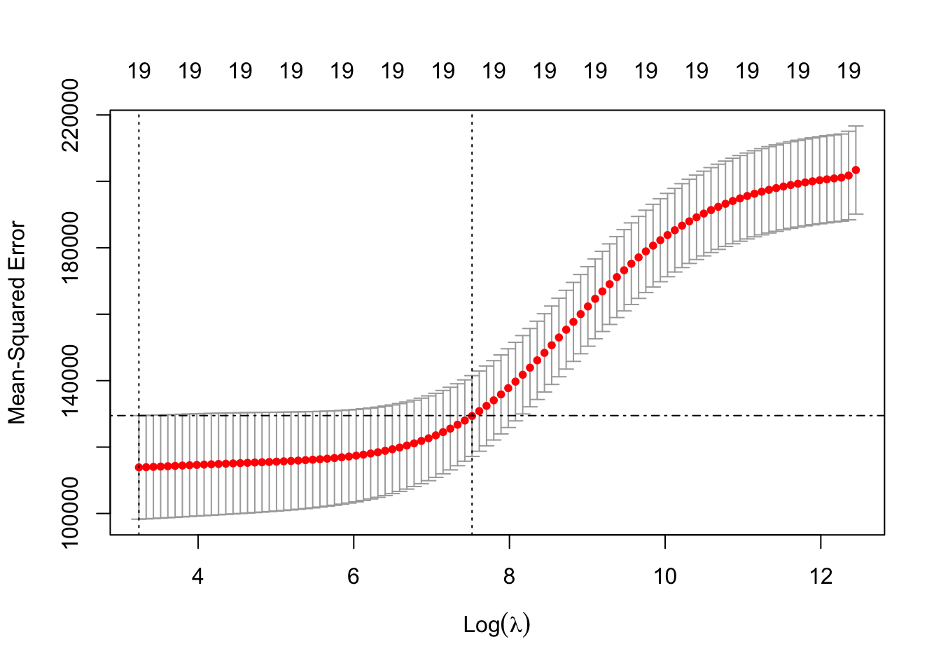

We can also plot the ridge regularisation paths and add the minimum-CV and 1-se \(\lambda\) values to the plot.

ridge = glmnet(x, y, alpha = 0)
plot(ridge, xvar = 'lambda')
abline(v = log(ridge.cv$lambda.min), lty = 3) # careful to use the log here  
                                              # and below
abline(v = log(ridge.cv$lambda.1se), lty = 3)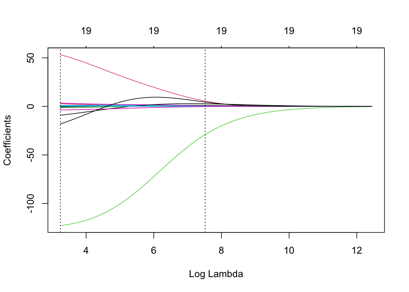

Important note: Any method/technique that relies on validation/cross-validation is subject to variability. If we re-run this code under a different random seed results will change.

Sparsifying the ridge coefficients?

One thing mentioned in Chapter 6.2 is that one can potentially consider some kind of post-hoc analysis in order to set some of the ridge coefficients equal to zero. A very simplistic approach is to just examine the ranking of the absolute coefficients and decide to use a “cutting-threshold”. We can use a combination of the commands sort() and abs() for this.

beta.1se =   coef( ridge.cv, s = 'lambda.1se' )[-1]
rank.coef = sort( abs( beta.1se ), decreasing = TRUE )
rank.coef

##  [1] 29.096663826  5.396487460  4.457548079  2.714623469  1.289060569
##  [6]  0.925962429  0.702915318  0.686866069  0.446840519  0.253594871
## [11]  0.235989099  0.102483884  0.071334608  0.068874010  0.067805863
## [16]  0.066114944  0.034359576  0.009201998  0.008746278

The last two coefficients are quite small, so we could potentially set these two equal to zero (setting a threshold of say, 0.01). Equivalently we may set a larger threshold of say, 1, in which case we would remove far more variables from the model. We could check whether this sparsification would offer any benefits in terms of predictive performance by, for example, using K-fold cross-validation to evaluate the standard ridge regression fit (using glmnet with alpha = 0) with the \(i\)th fold excluded, and predicting the output for the \(i\)th fold using predict (see ?predict.glmnet for details).

Lasso regression

As we did with ridge, we can use the function cv.glmnet() to find the min-CV \(\lambda\) and the 1 standard error (1-se) \(\lambda\) under lasso. The code is the following.

set.seed(1)
lasso.cv = cv.glmnet(x, y)
lasso.cv$lambda.min

## [1] 1.843343

lasso.cv$lambda.1se 

## [1] 69.40069

We see that in this case the 1-se \(\lambda\) is much larger than the min-CV \(\lambda\). This means that we expect the coefficients under 1-se \(\lambda\) to be much smaller (maybe exactly zero). Let’s have a look at the corresponding coefficients from the two models, rounding them to 3 decimal places.

round(cbind(
  coef(lasso.cv, s = 'lambda.min'),
  coef(lasso.cv, s = 'lambda.1se')),  
3)

## 20 x 2 sparse Matrix of class "dgCMatrix"
##                   s1      s1
## (Intercept)  142.878 127.957
## AtBat         -1.793   .    
## Hits           6.188   1.423
## HmRun          0.233   .    
## Runs           .       .    
## RBI            .       .    
## Walks          5.148   1.582
## Years        -10.393   .    
## CAtBat        -0.004   .    
## CHits          .       .    
## CHmRun         0.585   .    
## CRuns          0.764   0.160
## CRBI           0.388   0.337
## CWalks        -0.630   .    
## LeagueN       34.227   .    
## DivisionW   -118.981  -8.062
## PutOuts        0.279   0.084
## Assists        0.224   .    
## Errors        -2.436   .    
## NewLeagueN     .       .

Finally, lets plot the results of the object lasso.cv which we have created, and compare them to that of the lasso object generated in previous section.

par(mfrow=c(1,2))
plot(lasso.cv)
lasso = glmnet(x, y)
plot(lasso, xvar = 'lambda')
abline(v = log(lasso.cv$lambda.min), lty = 3) # careful to use the log here  
                                              # and below
abline(v = log(lasso.cv$lambda.1se), lty = 3)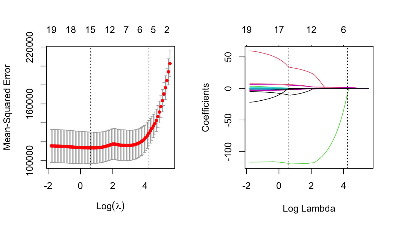

Notice now how the numbers across the top of the left-hand plot decrease as \(\lambda\) increases. This is indicating how many predictors are included for the corresponding \(\lambda\) value.

Comparing Predictive Performance for Different \(\lambda\)

We can investigate which of the two different \(\lambda\)-values (minimum-CV and 1-se) may be preferable in terms of predictive performance using the following code. Here, we split the data into a training and test set. We then use cross-validation to find minimum-CV \(\lambda\) and 1-se \(\lambda\), and use the resulting model to predict the response at the test data, comparing it to the actual response values by MSE. We then repeat this procedure many times using different splits in the data.

repetitions = 50
mse.1 = c()
mse.2 = c()

set.seed(1)                
for(i in 1:repetitions){
  
  # Step (i) data splitting
  training.obs = sample(1:263,  175)
  y.train = Hitters$Salary[training.obs]
  x.train = model.matrix(Salary~., Hitters[training.obs, ])[,-1]
  y.test = Hitters$Salary[-training.obs]
  x.test = model.matrix(Salary~., Hitters[-training.obs, ])[,-1]
  
  # Step (ii) training phase
  lasso.train = cv.glmnet(x.train, y.train)
  
  # Step (iii) generating predictions
  predict.1 = predict(lasso.train, x.test, s = 'lambda.min')
  predict.2 = predict(lasso.train, x.test, s = 'lambda.1se')
  
  # Step (iv) evaluating predictive performance
  mse.1[i] = mean((y.test-predict.1)^2)
  mse.2[i] = mean((y.test-predict.2)^2)
}

par(mfrow=c(1,1))
boxplot(mse.1, mse.2, names = c('min-CV lasso','1-se lasso'), 
        ylab = 'Test MSE', col = 7)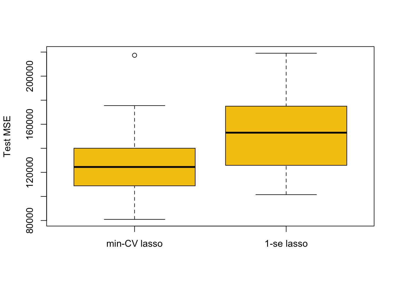

The approach based on min-CV is better, which makes sense as it minimised the cross-validation error (in cv.glmnet) in the first place. The 1-se \(\lambda\) can be of benefit in some cases for selecting models with fewer predictors that may be more interpretable. However, in applications where the 1-se \(\lambda\) is much larger than the min-CV \(\lambda\) (like here) we in general expect results as above.

References

Boyd, S., and L. Vandenberghe. 2009. Convex Optimization. 7th ed. Cambridge: Cambridge University Press.