Chapter 5 Model Search Methods
In this section, we consider some methods for selecting subsets of predictors.
5.1 Best Subset Selection
To perform best subset selection, we fit a separate least squares regression for each possible combination of the \(p\) predictors. This is often broken up into stages, as follows:
- Let \(M_0\) denote the null model which contains no predictors. This model simply predicts the sample mean of the response for each observation.
- For \(k = 1,2,\ldots,p\):
- Fit all \(\binom{p}{k}\) models1 that contain exactly \(k\) predictors.
- Pick the best among these \(\binom{p}{k}\) models and call it \(M_k\). Here best is defined as having the smallest RSS or largest \(R^2\).
- Select a single best model from among \(M_0, M_1,\ldots,M_p\) using cross-validated prediction error, \(C_p\) (AIC), BIC, or adjusted \(R^2\).
It is important to note that use of \(RSS\) or \(R^2\) in step 2 of the above algorithm is acceptable because the models all have an equal number of predictors. We can’t use \(RSS\) in step 3 because, as already discussed, \(RSS\) decreases monotonically as the number of predictors included in the model increases.
Cross-validation could also be used in step 2, but would be computationally more time-consuming as it would ultimately involve fitting all \(2^p\) possible models K times, each time excluding the \(i\)th fold when training and using the \(i\)th fold to calculate a prediction error. By only using cross-validation at step 3, we only need to fit \(p+1\) models K times.
An Illustation: Suppose we have three predictors \(X_1\), \(X_2\) and \(X_3\). In this case best subset selection works as follows:
\[\begin{align*} M_0: & \mbox{ intercept only (null model)}\\ C_1: & \begin{cases} X_1\\ X_2 \rightarrow \mbox{ lowest training } RSS \mbox{ within } C_1: \mbox{ make this } M_1 \\ X_3\\ \end{cases}\\ C_2: & \begin{cases} X_1, X_2 \rightarrow \mbox{ lowest training } RSS \mbox{ within } C_2: \mbox{ make this } M_2\\ X_1, X_3\\ X_2, X_3 \end{cases}\\ M_3: & ~X_1, X_2, X_3 \mbox{~ (full~model)} \end{align*}\]
We then choose one model among \(M_0, M_1, M_2, M_3\) either via validation/cross-validation, or based on \(C_p\), BIC, adjusted \(R^2\).
5.2 Forwards Stepwise Selection
For computational reasons, best subset selection cannot be applied with very large \(p\) as it needs to consider all \(2^p\) models. This is true even without using cross-validation which involves fitting the coefficients of at least some of the models K times. Best subset selection may also suffer from statistical problems when \(p\) is large. The larger the search space, the higher the chance of finding models which look good on (overfit) the training data, even though they might not have any predictive power on future data.
Forward stepwise selection is a computationally efficient alternative to best subset selection. This is because it considers a much smaller set of models. Forward stepwise selection works by starting with the model containing no predictors, and then adding one predictor at a time until all of the predictors are in the model. In particular, at each step the variable that gives the greatest additional improvement to the fit is added to the model. More formally, the algorithm proceeds as follows:
- Let \(M_0\) denote the null model which contains no predictors.
- For \(k = 0,1,...,p-1\):
- Consider all \(p-k\) models that augment the predictors in \(M_k\) with one additional predictor.
- Choose the best among these \(p-k\) models and call it \(M_{k+1}\). Here best is defined as having the smallest RSS or largest \(R^2\).
- Select a single best model from among \(M_0, M_1,\ldots,M_p\) using cross-validated prediction error, \(C_p\) (AIC), BIC, or adjusted \(R^2\).
An Illustation: Again, consider three predictors \(X_1\), \(X_2\) and \(X_3\). Forward stepwise selection works as follows:
\[\begin{align*} M_0: & \mbox{ intercept only (null model)}\\ C_1: & \begin{cases} X_1\\ X_2 \rightarrow \mbox{ lowest training } RSS \mbox{ within } C_1: \mbox{ make this } M_1\\ X_3\\ \end{cases}\\ C_2: & \begin{cases} X_1,X_2 \rightarrow \mbox{ lowest training } RSS \mbox{ within } C_2: \mbox{ make this } M_2\\ X_2, X_3 \end{cases}\\ M_3: & X_1, X_2, X_3 \mbox{ (full model)} \end{align*}\]
At the end we choose again one model among \(M_0, M_1, M_2, M_3\) based on validation/cross-validation, or based on \(C_p\), BIC, adjusted \(R^2\).
Some general comments:
- Best subset selection requires training \(2^p\) models, forward stepwise selection requires only \(1+\displaystyle\frac{p(p+1)}{2}\) comparisons.
- So for \(p=20\): best subset selection considers 1,048,576 models, whereas forward stepwise selection considers 211 models!
- There is cost to pay though for the gain in scalability. Forward stepwise selection can be sub-optimal in the sense that the models selected are not the best subset models.
- This is because the guided forward stepwise search at each step depends on the previously selected predictor.
- As an example, in the illustration above we had \(p=3\). The best possible one-variable model contained \(X_2\). It is quite possible that the best two-variable model contains the pair \((X_1,X_3)\), however, we did not consider this combination in the above algorithm.
- However, in practice best subset selection and forward stepwise selection perform quite similarly in terms of predictive accuracy.
5.3 Backwards Stepwise Selection
Backwards stepwise selection begins with the full model containing all \(p\) predictors, and iteratively removes the least useful predictor one-at-a-time.
- Let \(M_p\) denote the full model which contains all predictors.
- For \(k = p,p-1,\ldots,1\):
- Consider all \(k\) models that contain all but one of the predictors in \(M_k\), for a total of \(k-1\) predictors.
- Choose the best among these \(k\) models and call it \(M_{k-1}\). Here best is defined as having the smallest RSS or largest \(R^2\).
- Select a single best model from among \(M_0, M_1,\ldots,M_p\) using cross-validated prediction error, \(C_p\) (AIC), BIC, or adjusted \(R^2\).
Just like the forward algorithm, backward elimination requires only \(1+\displaystyle\frac{p(p+1)}{2}\) comparisons.
An Illustration: Again, consider three predictors \(X_1\), \(X_2\) and \(X_3\). Backwards stepwise selection works as follows:
\[\begin{align*} M_3: & X_1, X_2, X_3 \mbox{ (full model)}\\ C_2: & \begin{cases} X_1, X_2 \rightarrow \mbox{ lowest training } RSS \mbox{ within } C_2: \mbox{ make this } M_2\\ X_1, X_3\\ X_2, X_3 \end{cases}\\ C_1: & \begin{cases} X_1\\ X_2 \rightarrow \mbox{ lowest training } RSS \mbox{ within } C_1: \mbox{ make this } M_1\\ \end{cases}\\ M_0: & \mbox{ intercept only (null model)} \end{align*}\]
At the end we choose again one model among \(M_0, M_1, M_2, M_3\) based on cross-validation, or based on \(C_p\), BIC, adjusted \(R^2\).
5.3.1 Concluding Remarks
- Best subset, forward stepwise and backward stepwise selection approaches give similar but not identical results.
- Hybrid approaches that combine forward and backward steps also exist (but we will not cover these).
- Best subset and forward selection can be applied to some extent when \(n<p\), but only up to the model that contains \(n-1\) predictors. Backward selection cannot be applied when \(n<p\).
- The following practical demonstration and the practical classes will involve applying these methods to real data sets.
5.4 Practical Demonstration
In this practical demonstration we will start with an analysis of the Hitters dataset included in package ISLR. This dataset consists of 322 records of baseball players. The response variable is the players’ salary and the number of predictors is 19, including variables such as number of hits, years in the league and so forth.
5.4.1 Data handling
The first thing to do is to load the data by first installing package ISLR in R by typing install.packages('ISLR') (if you have already installed the package ignore this). Next we load the library and use ?Hitters which will open the help window in RStudio with information about the dataset.
library(ISLR)
?Hitters
Incidentally, recall that we can view the help file for any function or dataset in R by typing ? followed by the function or dataset, as above for dataset Hitters or below for function head. You will need to make use of this to increase your understanding of R - I will not be able to explain every detail of every function throughout these tutorials (although I will explain a lot), and you indeed will wish to vary the commands I call to do your own investigations!
To get a clearer picture of how the data looks we can use commands names(), head() and dim(). The first returns the names of the 20 variables, the second returns the first 6 rows (type ?head to see how to adjust this) and the third gives us the number of rows (sample size) and number of columns (1 response + 19 predictors).
names(Hitters) ## [1] "AtBat" "Hits" "HmRun" "Runs" "RBI" "Walks"
## [7] "Years" "CAtBat" "CHits" "CHmRun" "CRuns" "CRBI"
## [13] "CWalks" "League" "Division" "PutOuts" "Assists" "Errors"
## [19] "Salary" "NewLeague"head(Hitters) ## AtBat Hits HmRun Runs RBI Walks Years CAtBat CHits CHmRun
## -Andy Allanson 293 66 1 30 29 14 1 293 66 1
## -Alan Ashby 315 81 7 24 38 39 14 3449 835 69
## -Alvin Davis 479 130 18 66 72 76 3 1624 457 63
## -Andre Dawson 496 141 20 65 78 37 11 5628 1575 225
## -Andres Galarraga 321 87 10 39 42 30 2 396 101 12
## -Alfredo Griffin 594 169 4 74 51 35 11 4408 1133 19
## CRuns CRBI CWalks League Division PutOuts Assists Errors
## -Andy Allanson 30 29 14 A E 446 33 20
## -Alan Ashby 321 414 375 N W 632 43 10
## -Alvin Davis 224 266 263 A W 880 82 14
## -Andre Dawson 828 838 354 N E 200 11 3
## -Andres Galarraga 48 46 33 N E 805 40 4
## -Alfredo Griffin 501 336 194 A W 282 421 25
## Salary NewLeague
## -Andy Allanson NA A
## -Alan Ashby 475.0 N
## -Alvin Davis 480.0 A
## -Andre Dawson 500.0 N
## -Andres Galarraga 91.5 N
## -Alfredo Griffin 750.0 Adim(Hitters)## [1] 322 20Prior to proceeding to any analysis we must check whether the data contains any missing values. To do this we can use a combination of the commands sum() and is.na(). We find that we have 59 missing Salary entries. To remove these 59 rows we make use of the command na.omit() and then double-check.
sum( is.na( Hitters ) ) # checks for missing data in the entire dataframe.## [1] 59sum( is.na( Hitters$Salary ) ) # checks for missing data in the response only.## [1] 59Hitters = na.omit( Hitters ) # removes entries to the dataframe with any data
# missing.
dim( Hitters )## [1] 263 20sum( is.na( Hitters ) ) # check that there is now no ## [1] 0 # missing data in the dataframe.5.4.2 Best Subset Selection
Now we are ready to start with best subset selection. There are different packages in R which perform best subset as well as stepwise selections. We will use the function regsubsets() from library leaps (again install.packages('leaps') is needed if not already installed). regsubsets() essentially performs step 2 of the algorithm presented in Section 5.1, although yields results that make step 3 relatively straightforward. Note that the . part of Salary~. indicates that we wish to consider all possible predictors in the subset selection method. We will store the results from best subset in an object called best (any name would do) and summarize the results via summary(), which outputs the best models of different dimensionality.
library(leaps)
best = regsubsets(Salary~., Hitters)
summary(best)
## Subset selection object
## Call: regsubsets.formula(Salary ~ ., Hitters)
## 19 Variables (and intercept)
## Forced in Forced out
## AtBat FALSE FALSE
## Hits FALSE FALSE
## HmRun FALSE FALSE
## Runs FALSE FALSE
## RBI FALSE FALSE
## Walks FALSE FALSE
## Years FALSE FALSE
## CAtBat FALSE FALSE
## CHits FALSE FALSE
## CHmRun FALSE FALSE
## CRuns FALSE FALSE
## CRBI FALSE FALSE
## CWalks FALSE FALSE
## LeagueN FALSE FALSE
## DivisionW FALSE FALSE
## PutOuts FALSE FALSE
## Assists FALSE FALSE
## Errors FALSE FALSE
## NewLeagueN FALSE FALSE
## 1 subsets of each size up to 8
## Selection Algorithm: exhaustive
## AtBat Hits HmRun Runs RBI Walks Years CAtBat CHits CHmRun CRuns CRBI
## 1 ( 1 ) " " " " " " " " " " " " " " " " " " " " " " "*"
## 2 ( 1 ) " " "*" " " " " " " " " " " " " " " " " " " "*"
## 3 ( 1 ) " " "*" " " " " " " " " " " " " " " " " " " "*"
## 4 ( 1 ) " " "*" " " " " " " " " " " " " " " " " " " "*"
## 5 ( 1 ) "*" "*" " " " " " " " " " " " " " " " " " " "*"
## 6 ( 1 ) "*" "*" " " " " " " "*" " " " " " " " " " " "*"
## 7 ( 1 ) " " "*" " " " " " " "*" " " "*" "*" "*" " " " "
## 8 ( 1 ) "*" "*" " " " " " " "*" " " " " " " "*" "*" " "
## CWalks LeagueN DivisionW PutOuts Assists Errors NewLeagueN
## 1 ( 1 ) " " " " " " " " " " " " " "
## 2 ( 1 ) " " " " " " " " " " " " " "
## 3 ( 1 ) " " " " " " "*" " " " " " "
## 4 ( 1 ) " " " " "*" "*" " " " " " "
## 5 ( 1 ) " " " " "*" "*" " " " " " "
## 6 ( 1 ) " " " " "*" "*" " " " " " "
## 7 ( 1 ) " " " " "*" "*" " " " " " "
## 8 ( 1 ) "*" " " "*" "*" " " " " " "The asterisks * indicate variables which are included in model \(M_k, k = 1,...,19\) as discussed in the subset selection algorithm of Section 5.1. For instance, we see that for the model with one predictor that variable is CRBI, while for the model with four predictors the selected variables are Hits, CRBI, DivisionW and PutOuts. As we see the summary() command displayed output up to the best model with 8 predictors; this is the default option in regsubsets(). To change this we can use the extra argument nvmax. Below we re-run the command for all best models (19 in total). Now we also store the output of summary() in an object called results and further investigate what this contains via names(). As we can see there is a lot of useful information! Of particular use to us, we can see that it returns \(R^2\), RSS, adjusted-\(R^2\), \(C_p\) and BIC. We can easily extract these quantities; for instance below we see the \(R^2\) values for the 19 models.
best = regsubsets(Salary~., data = Hitters, nvmax = 19)
results = summary(best)
names(results)
## [1] "which" "rsq" "rss" "adjr2" "cp" "bic" "outmat" "obj"results$rsq## [1] 0.3214501 0.4252237 0.4514294 0.4754067 0.4908036 0.5087146 0.5141227
## [8] 0.5285569 0.5346124 0.5404950 0.5426153 0.5436302 0.5444570 0.5452164
## [15] 0.5454692 0.5457656 0.5459518 0.5460945 0.5461159Lets store these quantities as separate objects. We can also stack them together into one matrix as done below and see the values.
RSS = results$rss
r2 = results$rsq
Cp = results$cp
BIC = results$bic
Adj_r2 = results$adjr2

cbind(RSS, r2, Cp, BIC, Adj_r2)
## RSS r2 Cp BIC Adj_r2
## [1,] 36179679 0.3214501 104.281319 -90.84637 0.3188503
## [2,] 30646560 0.4252237 50.723090 -128.92622 0.4208024
## [3,] 29249297 0.4514294 38.693127 -135.62693 0.4450753
## [4,] 27970852 0.4754067 27.856220 -141.80892 0.4672734
## [5,] 27149899 0.4908036 21.613011 -144.07143 0.4808971
## [6,] 26194904 0.5087146 14.023870 -147.91690 0.4972001
## [7,] 25906548 0.5141227 13.128474 -145.25594 0.5007849
## [8,] 25136930 0.5285569 7.400719 -147.61525 0.5137083
## [9,] 24814051 0.5346124 6.158685 -145.44316 0.5180572
## [10,] 24500402 0.5404950 5.009317 -143.21651 0.5222606
## [11,] 24387345 0.5426153 5.874113 -138.86077 0.5225706
## [12,] 24333232 0.5436302 7.330766 -133.87283 0.5217245
## [13,] 24289148 0.5444570 8.888112 -128.77759 0.5206736
## [14,] 24248660 0.5452164 10.481576 -123.64420 0.5195431
## [15,] 24235177 0.5454692 12.346193 -118.21832 0.5178661
## [16,] 24219377 0.5457656 14.187546 -112.81768 0.5162219
## [17,] 24209447 0.5459518 16.087831 -107.35339 0.5144464
## [18,] 24201837 0.5460945 18.011425 -101.86391 0.5126097
## [19,] 24200700 0.5461159 20.000000 -96.30412 0.5106270We know that RSS should steadily decrease and that \(R^2\) increase as we add predictors. Lets check that by plotting the values of RSS and \(R^2\). We would like to have the two plots next to each other, so will make use of the command par(mfrow()), with the c(1, 2) indicating we require the plotting window to contain 1 row and 2 columns, before calling the command plot().
par(mfrow = c(1, 2))
plot(RSS, xlab = "Number of Predictors", ylab = "RSS",
     type = "l", lwd = 2)
plot(r2, xlab = "Number of Predictors", ylab = "R-square",
     type = "l", lwd = 2)
Results are as expected. Above the argument type = 'l' is used for the lines to appear (otherwise by default R would simply plot the points) and the argument lwd controls the thickness of the lines. Plots in R are very customizable (type ?par to see all available options).
Now let us find how many predictors are included in the optimal models under \(Cp\), BIC and adjusted-\(R^2\) and produce some plots illustrating this information.
which.min(Cp)## [1] 10which.min(BIC)## [1] 6which.max(Adj_r2)## [1] 11par(mfrow = c(1, 3))
plot(Cp, xlab = "Number of Predictors", ylab = "Cp",
type = 'l', lwd = 2)
points(10, Cp[10], col = "red", cex = 2, pch = 8, lwd = 2)
plot(BIC, xlab = "Number of Predictors", ylab = "BIC",
type = 'l', lwd = 2)
points(6, BIC[6], col = "red", cex = 2, pch = 8, lwd = 2)
plot(Adj_r2, xlab = "Number of Predictors", ylab = "Adjusted RSq",
type = "l", lwd = 2)
points(11, Adj_r2[11], col = "red", cex = 2, pch = 8, lwd = 2)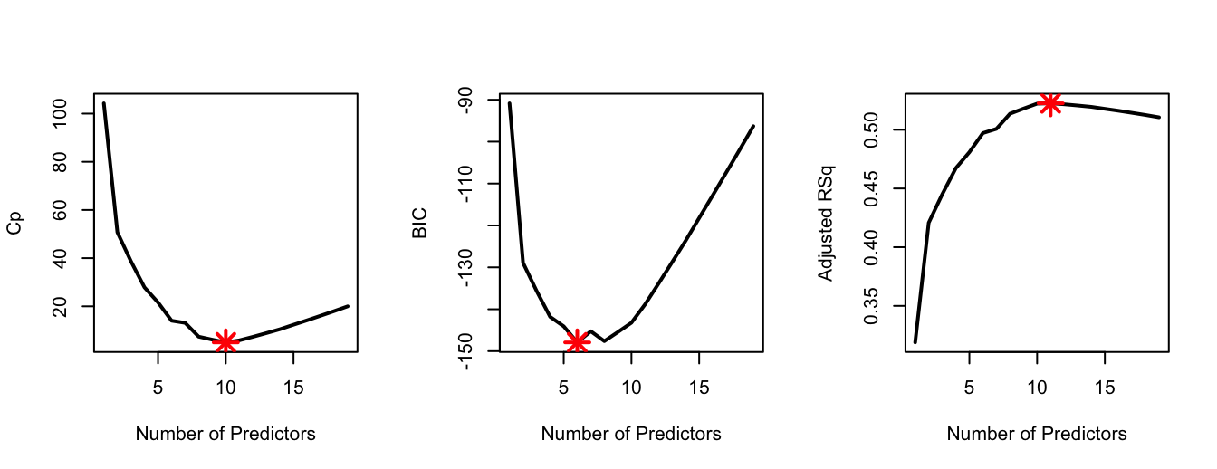
\(Cp\) and adjusted-\(R^2\) select 10 and 11 predictors respectively, while the optimal BIC model has only 6 predictors. In the code above we use the command points() to highlight the optimal model; the first two arguments of this command correspond to x-axis and y-axis co-ordinates. So, for example, we know that the optimal \(C_p\) model is the one with 10 predictors; therefore the first argument is set to 10 and the second argument is set to Cp[10] (i.e., \(C_p\) at its minimum).
The regsubsets() in-built function for plotting the results is very convenient when the output from summary() is difficult to read due to there being many possible predictors. Below we see the visualisation for the BIC models. Remark: Because previously we used par(mfrow(1,3)) we have to either close the plotting panel by typing dev.off() (this returns the window plot to the default state), or respecifying the window splitting using par( mfrow = c(1,1) ).
plot(best, scale = "bic")
The top row corresponds to the best model, while the bottom row to the worst model according to the chosen criterion. White squares correspond to variables that are excluded under each model.
Finally, we extract the model coefficients for any model we choose via the command coef. For instance, the best models under each approach are the following.
coef(best,10) # Cp## (Intercept) AtBat Hits Walks CAtBat CRuns
## 162.5354420 -2.1686501 6.9180175 5.7732246 -0.1300798 1.4082490
## CRBI CWalks DivisionW PutOuts Assists
## 0.7743122 -0.8308264 -112.3800575 0.2973726 0.2831680coef(best,6) # BIC## (Intercept) AtBat Hits Walks CRBI DivisionW
## 91.5117981 -1.8685892 7.6043976 3.6976468 0.6430169 -122.9515338
## PutOuts
## 0.2643076coef(best,11) # adj-Rsq## (Intercept) AtBat Hits Walks CAtBat CRuns
## 135.7512195 -2.1277482 6.9236994 5.6202755 -0.1389914 1.4553310
## CRBI CWalks LeagueN DivisionW PutOuts Assists
## 0.7852528 -0.8228559 43.1116152 -111.1460252 0.2894087 0.26882775.4.3 Forward Stepwise Selection
We can use the same function to also perform forward or backward selection by only changing one of its arguments. Forward selection can be implemented in the following way.
fwd = regsubsets(Salary~., data = Hitters, nvmax = 19,
                 method = "forward")
summary(fwd)
## Subset selection object
## Call: regsubsets.formula(Salary ~ ., data = Hitters, nvmax = 19, method = "forward")
## 19 Variables (and intercept)
## Forced in Forced out
## AtBat FALSE FALSE
## Hits FALSE FALSE
## HmRun FALSE FALSE
## Runs FALSE FALSE
## RBI FALSE FALSE
## Walks FALSE FALSE
## Years FALSE FALSE
## CAtBat FALSE FALSE
## CHits FALSE FALSE
## CHmRun FALSE FALSE
## CRuns FALSE FALSE
## CRBI FALSE FALSE
## CWalks FALSE FALSE
## LeagueN FALSE FALSE
## DivisionW FALSE FALSE
## PutOuts FALSE FALSE
## Assists FALSE FALSE
## Errors FALSE FALSE
## NewLeagueN FALSE FALSE
## 1 subsets of each size up to 19
## Selection Algorithm: forward
## AtBat Hits HmRun Runs RBI Walks Years CAtBat CHits CHmRun CRuns CRBI
## 1 ( 1 ) " " " " " " " " " " " " " " " " " " " " " " "*"
## 2 ( 1 ) " " "*" " " " " " " " " " " " " " " " " " " "*"
## 3 ( 1 ) " " "*" " " " " " " " " " " " " " " " " " " "*"
## 4 ( 1 ) " " "*" " " " " " " " " " " " " " " " " " " "*"
## 5 ( 1 ) "*" "*" " " " " " " " " " " " " " " " " " " "*"
## 6 ( 1 ) "*" "*" " " " " " " "*" " " " " " " " " " " "*"
## 7 ( 1 ) "*" "*" " " " " " " "*" " " " " " " " " " " "*"
## 8 ( 1 ) "*" "*" " " " " " " "*" " " " " " " " " "*" "*"
## 9 ( 1 ) "*" "*" " " " " " " "*" " " "*" " " " " "*" "*"
## 10 ( 1 ) "*" "*" " " " " " " "*" " " "*" " " " " "*" "*"
## 11 ( 1 ) "*" "*" " " " " " " "*" " " "*" " " " " "*" "*"
## 12 ( 1 ) "*" "*" " " "*" " " "*" " " "*" " " " " "*" "*"
## 13 ( 1 ) "*" "*" " " "*" " " "*" " " "*" " " " " "*" "*"
## 14 ( 1 ) "*" "*" "*" "*" " " "*" " " "*" " " " " "*" "*"
## 15 ( 1 ) "*" "*" "*" "*" " " "*" " " "*" "*" " " "*" "*"
## 16 ( 1 ) "*" "*" "*" "*" "*" "*" " " "*" "*" " " "*" "*"
## 17 ( 1 ) "*" "*" "*" "*" "*" "*" " " "*" "*" " " "*" "*"
## 18 ( 1 ) "*" "*" "*" "*" "*" "*" "*" "*" "*" " " "*" "*"
## 19 ( 1 ) "*" "*" "*" "*" "*" "*" "*" "*" "*" "*" "*" "*"
## CWalks LeagueN DivisionW PutOuts Assists Errors NewLeagueN
## 1 ( 1 ) " " " " " " " " " " " " " "
## 2 ( 1 ) " " " " " " " " " " " " " "
## 3 ( 1 ) " " " " " " "*" " " " " " "
## 4 ( 1 ) " " " " "*" "*" " " " " " "
## 5 ( 1 ) " " " " "*" "*" " " " " " "
## 6 ( 1 ) " " " " "*" "*" " " " " " "
## 7 ( 1 ) "*" " " "*" "*" " " " " " "
## 8 ( 1 ) "*" " " "*" "*" " " " " " "
## 9 ( 1 ) "*" " " "*" "*" " " " " " "
## 10 ( 1 ) "*" " " "*" "*" "*" " " " "
## 11 ( 1 ) "*" "*" "*" "*" "*" " " " "
## 12 ( 1 ) "*" "*" "*" "*" "*" " " " "
## 13 ( 1 ) "*" "*" "*" "*" "*" "*" " "
## 14 ( 1 ) "*" "*" "*" "*" "*" "*" " "
## 15 ( 1 ) "*" "*" "*" "*" "*" "*" " "
## 16 ( 1 ) "*" "*" "*" "*" "*" "*" " "
## 17 ( 1 ) "*" "*" "*" "*" "*" "*" "*"
## 18 ( 1 ) "*" "*" "*" "*" "*" "*" "*"
## 19 ( 1 ) "*" "*" "*" "*" "*" "*" "*"The analysis will then be essentially identical to the previous analysis for best subset selection.
One interesting thing to check is whether the results from best subset and forward stepwise selection are in agreement (we know that this will not necessarily be the case). For example, let’s have a look at the models with 6 and 7 predictors.
coef(best, 6)## (Intercept) AtBat Hits Walks CRBI DivisionW
## 91.5117981 -1.8685892 7.6043976 3.6976468 0.6430169 -122.9515338
## PutOuts
## 0.2643076coef(fwd, 6)## (Intercept) AtBat Hits Walks CRBI DivisionW
## 91.5117981 -1.8685892 7.6043976 3.6976468 0.6430169 -122.9515338
## PutOuts
## 0.2643076coef(best, 7)## (Intercept) Hits Walks CAtBat CHits CHmRun
## 79.4509472 1.2833513 3.2274264 -0.3752350 1.4957073 1.4420538
## DivisionW PutOuts
## -129.9866432 0.2366813coef(fwd, 7)## (Intercept) AtBat Hits Walks CRBI CWalks
## 109.7873062 -1.9588851 7.4498772 4.9131401 0.8537622 -0.3053070
## DivisionW PutOuts
## -127.1223928 0.2533404The results for the model with 6 predictors are in agreement (which is good to know because this would be one of the three models one would likely select), but as we see the results for the models with 7 predictors are different.
5.4.4 Best Subset Selection: Validation
In this section, we consider applying best subset selection not based on model selection criteria but using the validation approach.
As we know, for validation (and cross-validation) we need to be able to predict from our linear models. Unfortunately, regsubsets() doesn’t have its own built-in function for that (most similar types of R functions have). You are welcome to try writing your own code for this step, but it is beyond the scope of the course. For the purposes of performing subset selection by validation in this course, we will just make use of the function predict.regsubsets below which will do the predictions for us. The important aspects of the function are the arguments. object should be the result of a call to the function regsubsets() (for example the object best in Section 5.4.2 or fwd in Section 5.4.3), newdata should be a dataframe of data at which we wish to predict at, and id indicates that we wish to use the resulting model from regsubsets with id number of predictors (so in this case could range from 1,2,…19). The output is the response prediction for each combination of inputs. Note that if you wish to use this function in your own code you will need to define it by copy and pasting this code segment.
predict.regsubsets = function(object, newdata, id, ...){
  form = as.formula(object$call[[2]])
  mat = model.matrix(form, newdata)
  coefi = coef(object, id = id)
  xvars = names(coefi)
  mat[, xvars]%*%coefi
}
The validation approach is based on splitting the data once into a training sample and a validation or testing sample. We also need to decide how to split the data. A common approach is to use 2/3 of the sample for training and 1/3 of the sample for testing (although it does not have to be so).
Note the first line: set.seed. If we removed this command, then every time we ran the following code we could get different results (for example, variables selected) due to the effect of the random sample (do feel free to try this, or alternatively changing the seed number). set.seed ensures a particular random state for any particular integer value, thus making the code reproducible (i.e. the same every time).
set.seed(10)          # for the results to be reproducible
dim(Hitters)
## [1] 263 20training.obs = sample(1:263, 175)
Hitters.train = Hitters[training.obs, ]
Hitters.test = Hitters[-training.obs, ]
dim(Hitters.train)## [1] 175 20dim(Hitters.test)## [1] 88 20Validation is then executed as follows. We first apply regsubsets() to the training set. By doing so note how we are only using the training data for both steps 2 and 3 of the algorithm in Section 5.1.
best.val = regsubsets(Salary~., data = Hitters.train, nvmax = 19)Then we create an empty vector called val.error where we will store the 19 (because we have 19 models) validation MSEs. We then use a for loop inside which we (i) generate predictions using predict.regsubsets() and (ii) calculate the validation MSEs. At the end we just locate which model produces the lowest MSE. The code is the following.
val.error<-c()
for(i in 1:19){
  pred = predict.regsubsets(best.val, Hitters.test, i)
  val.error[i] = mean((Hitters.test$Salary - pred)^2)
}

val.error
## [1] 199324.8 184215.9 196949.2 192709.1 180806.0 179388.2 178929.9 176754.4
## [9] 177029.2 163013.2 165134.5 164986.7 166072.1 164983.9 164890.7 165144.4
## [17] 164983.7 164962.6 164959.9which.min(val.error)## [1] 10In this instance we see that the model with 10 predictors is selected as the best. This was also the model selected by \(C_p\) in Section 5.4.2.
5.4.5 What about inference?
Note that the aim of subset selection is to find which predictors should be included within our model, not to identify the specific model (including coefficient values). Therefore, it is important to note that there is a final step to fitting a model by validation, and that is to train the same 10-predictor model to the entire data. This will yield different coefficient values to the current coefficients. The current coefficients should not be used because these were “learned” from the reduced training sample (that is, we didn’t use all of the available data).
For the purpose of fitting a specific model (with specified predictors) we use the command lm() in R.
coef(best.val, 10) # Check which variables to use in the lm.## (Intercept) AtBat Hits Runs Walks CAtBat
## -21.6323918 -0.7961450 4.5874937 -3.1211583 7.5830718 -0.1058408
## CRuns CRBI CWalks DivisionW PutOuts
## 1.9895304 0.3010303 -1.1736748 -121.3385526 0.1989660ls10 = lm(Salary ~ AtBat + Hits + Runs + Walks + CAtBat + CRuns + CRBI
+ CWalks + Division + PutOuts, data = Hitters)As we have seen the output from regsubsets() relates to the model selection procedure; i.e. we get the values of \(Cp\), BIC, adjusted-\(R^2\). We can also extract model specific regression coefficients via the command coef(). However, the lm object above is required for quantities such as standard errors, confidence and prediction intervals etc., for example, recalling that summary() provides a summary, and confint() provides confidence intervals. In addition, we can now use this model for prediction purposes using the built-in predict function for linear models (which is distinct to the predict.regsubsets function we defined above).
summary(ls10)##
## Call:
## lm(formula = Salary ~ AtBat + Hits + Runs + Walks + CAtBat +
## CRuns + CRBI + CWalks + Division + PutOuts, data = Hitters)
##
## Residuals:
## Min 1Q Median 3Q Max
## -927.60 -177.70 -30.03 142.91 1986.30
##
## Coefficients:
## Estimate Std. Error t value Pr(>|t|)
## (Intercept) 144.30288 66.52508 2.169 0.031007 *
## AtBat -1.84992 0.52681 -3.512 0.000528 ***
## Hits 7.64658 1.82552 4.189 0.0000388 ***
## Runs -2.92542 2.33580 -1.252 0.211576
## Walks 6.28202 1.68895 3.719 0.000246 ***
## CAtBat -0.12749 0.05751 -2.217 0.027517 *
## CRuns 1.45072 0.41373 3.506 0.000537 ***
## CRBI 0.66823 0.20074 3.329 0.001002 **
## CWalks -0.80479 0.26367 -3.052 0.002515 **
## DivisionW -117.14522 39.33350 -2.978 0.003182 **
## PutOuts 0.27111 0.07406 3.661 0.000307 ***
## ---
## Signif. codes: 0 '***' 0.001 '**' 0.01 '*' 0.05 '.' 0.1 ' ' 1
##
## Residual standard error: 312.8 on 252 degrees of freedom
## Multiple R-squared: 0.5375, Adjusted R-squared: 0.5191
## F-statistic: 29.29 on 10 and 252 DF, p-value: < 0.00000000000000022confint(ls10, 1:11)## 2.5 % 97.5 %
## (Intercept) 13.2868988 275.31885341
## AtBat -2.8874302 -0.81240354
## Hits 4.0513571 11.24181209
## Runs -7.5256017 1.67476709
## Walks 2.9557696 9.60827296
## CAtBat -0.2407504 -0.01423684
## CRuns 0.6359135 2.26553592
## CRBI 0.2728907 1.06357743
## CWalks -1.3240670 -0.28550387
## DivisionW -194.6094923 -39.68094337
## PutOuts 0.1252518 0.41696960test.data <- data.frame( "AtBat" = 322, "Hits" = 90, "HmRun" = 14,
"Runs" = 40, "RBI" = 22, "Walks" = 40,
"Years" = 4, "CAtBat" = 3000, "CHits" = 830,
"CHMRun" = 100, "CRuns" = 250, "CRBI" = 600,
"CWalks" = 300, "League" = "N", "Division" = "W",
"PutOuts" = 600, "Assists" = 60, "Errors" = 7,
"newLeague" = "N" )
predict( ls10, newdata = test.data )## 1
## 556.31275.4.6 Variance of selection based on validation
When using validation and cross-validation for best subset selection (or any stepwise method) it is important to understand that results depend on the random splitting between training and testing samples. This is generally a drawback which is not discussed a lot, especially for the simple validation approach. The below code implements the validation approach presented previously but now starting from 50 different random seeds, storing the number of predictors in the selected model each time.
min.valid = c()

for(n in 1:50){
  set.seed(n)
  training.obs = sample(1:263, 175)
  Hitters.train = Hitters[training.obs,  ]
  Hitters.test = Hitters[-training.obs,  ]

  best.val = regsubsets(Salary~., data = Hitters.train, nvmax = 19)

  val.error<-c()
  for(i in 1:19){
    pred = predict.regsubsets(best.val, Hitters.test, i)
    val.error[i] = mean((Hitters.test$Salary - pred)^2)
  }
  val.error
  min.valid[n] = which.min(val.error)
}
The histogram below shows that the final selection of the best model can vary a lot, even in terms of the number of predictors! Note that in addition, the histogram doesn’t tell the whole story because each time, say, a 10-predictor model is chosen, it may be choosing different predictors. In this case we can see that the validation method is most often choosing a model with 8, 9 or 10 predictors.
hist(min.valid, col = 3, breaks = seq( from = 0.5, to = 19.5, length = 20 ),
     xlab = 'Number of Predictors',
     main = 'Best Subset Selection with validation')
abline(v = mean(min.valid), col = 2, lwd = 4)
legend('topright', legend=c('Average selection'),bty = 'n', lty = 1,
       lwd = 4, col = 2)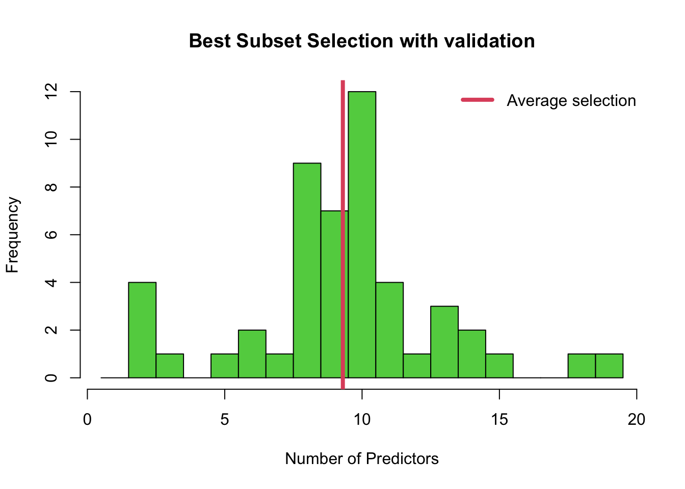
5.4.7 Cross-validation
Now lets turn our attention to the K-fold cross-validation (CV) approach. This procedure is generally preferable to simple validation because it utilizes the entire sample for training as well as for testing.
In contrast to the application of validation in Section 5.4.4, where we used the training data for both steps 2 and 3 of the algorithm presented in Section 5.1, we here use the full dataset in the initial regsubsets() command (step 2), and cross-validation for step 3 only. Therefore step 2 proceeds as before:
best = regsubsets(Salary~., data = Hitters, nvmax = 19)Since step 3 involves fitting models with specified predictors, we need to once again use the lm() function in R. Since this would involve manually specifying 19 models using lm(), we will instead demonstrate how to obtain a K-fold cross-validation error for just 3 of the models suggested by regsubsets() only.
In particular, we are going to answer the following question…which of the different models chosen under \(C_p\), BIC and adjusted \(R^2\) respectively in Section 5.4.2 should we choose? Recall \(C_p\) yielded the model with 10 variables, BIC the one with 6, and adjusted \(R^2\) the one with 11. Therefore, we will calculate the K-fold cross-validation error of the models with 6, 10 and 11 variables suggested by regsubsets() only. Let’s remind ourselves of the variables in those three models:
coef(best,10) # Cp## (Intercept) AtBat Hits Walks CAtBat CRuns
## 162.5354420 -2.1686501 6.9180175 5.7732246 -0.1300798 1.4082490
## CRBI CWalks DivisionW PutOuts Assists
## 0.7743122 -0.8308264 -112.3800575 0.2973726 0.2831680coef(best,6) # BIC## (Intercept) AtBat Hits Walks CRBI DivisionW
## 91.5117981 -1.8685892 7.6043976 3.6976468 0.6430169 -122.9515338
## PutOuts
## 0.2643076coef(best,11) # adj-Rsq## (Intercept) AtBat Hits Walks CAtBat CRuns
## 135.7512195 -2.1277482 6.9236994 5.6202755 -0.1389914 1.4553310
## CRBI CWalks LeagueN DivisionW PutOuts Assists
## 0.7852528 -0.8228559 43.1116152 -111.1460252 0.2894087 0.2688277Linear models based on the whole training set would be constructed as follows:
ls10 = lm(Salary ~ AtBat + Hits + Walks + CAtBat + CRuns + CRBI + CWalks +
          Division + PutOuts + Assists, data = Hitters)
ls6 = lm(Salary ~ AtBat + Hits + Walks + CRBI + Division + PutOuts,
         data = Hitters)
ls11 = lm(Salary ~ AtBat + Hits + Walks + CAtBat + CRuns + CRBI + CWalks +
          + League + Division + PutOuts + Assists, data = Hitters)
Now we turn to calculating K-fold cross-validation errors for these models. A first question is how many folds to use. Common choices in practice are 5 and 10, leading to 5-fold and 10-fold CV. In this example we will use 10 folds. Of course, often the sample size n will not be perfectly divisable by K (as in our case where n=263 and K=10). This does not matter, since it is not a problem if some folds have fewer observations.
Lets see how we can create folds in R. First we need to form an indicator vector with length equal to 263 containing the numbers 1,2,3,4,5,6,7,8,9,10 roughly the same number of times. This can be done by combining the commands cut() and seq() in R as below. The command table() then tabulates how many of each integer are present in the resulting vector.
k = 10
folds = cut(1:263, breaks=10, labels=FALSE)
folds
## [1] 1 1 1 1 1 1 1 1 1 1 1 1 1 1 1 1 1 1 1 1 1 1 1 1 1
## [26] 1 1 2 2 2 2 2 2 2 2 2 2 2 2 2 2 2 2 2 2 2 2 2 2 2
## [51] 2 2 2 3 3 3 3 3 3 3 3 3 3 3 3 3 3 3 3 3 3 3 3 3 3
## [76] 3 3 3 3 4 4 4 4 4 4 4 4 4 4 4 4 4 4 4 4 4 4 4 4 4
## [101] 4 4 4 4 4 5 5 5 5 5 5 5 5 5 5 5 5 5 5 5 5 5 5 5 5
## [126] 5 5 5 5 5 5 5 6 6 6 6 6 6 6 6 6 6 6 6 6 6 6 6 6 6
## [151] 6 6 6 6 6 6 6 6 7 7 7 7 7 7 7 7 7 7 7 7 7 7 7 7 7
## [176] 7 7 7 7 7 7 7 7 7 8 8 8 8 8 8 8 8 8 8 8 8 8 8 8 8
## [201] 8 8 8 8 8 8 8 8 8 8 9 9 9 9 9 9 9 9 9 9 9 9 9 9 9
## [226] 9 9 9 9 9 9 9 9 9 9 9 10 10 10 10 10 10 10 10 10 10 10 10 10 10
## [251] 10 10 10 10 10 10 10 10 10 10 10 10 10table(folds)## folds
## 1 2 3 4 5 6 7 8 9 10
## 27 26 26 26 27 26 26 26 26 27It is then very important to randomly re-shuffle this vector, because we do not want the fold creation procedure to be deterministic. We can do this very easily in R using once again the command sample().
set.seed(2)
folds = sample(folds)
folds
## [1] 8 10 8 7 3 5 3 6 9 2 3 4 5 9 7 2 10 5 7 6 2 10 8 6 4
## [26] 1 5 8 7 5 10 4 5 10 8 8 1 5 9 2 2 10 8 10 1 1 7 9 2 6
## [51] 5 8 3 4 8 2 1 6 8 10 5 7 2 3 7 7 1 1 7 3 9 8 4 3 6
## [76] 7 5 5 10 2 5 6 2 1 4 5 9 1 3 3 8 3 10 8 6 1 2 6 1 4
## [101] 9 6 4 10 9 1 9 7 9 8 4 8 6 1 10 2 10 10 7 9 3 9 4 4 5
## [126] 6 10 3 9 2 8 8 6 2 2 6 1 9 1 10 7 4 2 4 8 5 8 1 6 3
## [151] 1 10 10 1 3 3 3 7 3 4 2 9 4 6 8 9 7 2 1 7 4 3 5 7 8
## [176] 4 9 7 9 5 2 1 1 6 4 4 5 10 6 5 1 10 9 7 3 1 5 2 7 7
## [201] 4 6 7 10 3 6 5 10 4 9 9 5 7 7 2 6 9 5 5 3 2 3 5 5 9
## [226] 3 6 1 1 9 8 6 8 9 10 4 4 10 10 5 2 3 3 6 3 4 10 9 6 2
## [251] 1 8 6 7 8 4 2 8 1 10 2 7 4Finally, we need to create a matrix this time with K=10 rows and 3 columns. The validation MSEs of the folds for model ls10 will be stored in the first column of this matrix, the validation MSEs of the folds for model ls6 will be stored in the second column of this matrix, and the validation MSEs of the folds for model ls11 will be stored in the final column.
cv.errors = matrix(NA, nrow = k, ncol = 3,
                   dimnames = list(NULL, c("ls10", "ls6", "ls11")))
cv.errors
## ls10 ls6 ls11
## [1,] NA NA NA
## [2,] NA NA NA
## [3,] NA NA NA
## [4,] NA NA NA
## [5,] NA NA NA
## [6,] NA NA NA
## [7,] NA NA NA
## [8,] NA NA NA
## [9,] NA NA NA
## [10,] NA NA NAAbove NA means “not available”. The NA entries will be replaced with the MSEs as the loop below progresses. The part dimnames = list(NULL, c("ls10", "ls6", "ls11")) just assigns no names to the rows and names the columns "ls10", "ls6" and "ls11" respectively.
Now for calculating the cross-validation errors we will need a for loop to loop over the folds. The important part is to understand what data = Hitters[folds!=i, ] is doing. In R != means “not equal”. So for example when i=1 we discard the rows of Hitter for which the corresponding fold vector equals 1. We then predict only for the rows for which the fold vector equals i (in Hitters[folds==i, ] and Hitters$Salary[folds==i]). We then store each validation MSE in the appropriate row and column of cv.errors.
for(i in 1:k){
ls10 = lm(Salary ~ AtBat + Hits + Walks + CAtBat + CRuns + CRBI + CWalks +
          Division + PutOuts + Assists, data = Hitters[folds!=i, ] )
ls6 = lm(Salary ~ AtBat + Hits + Walks + CRBI + Division + PutOuts,
         data = Hitters[folds!=i, ])
ls11 = lm(Salary ~ AtBat + Hits + Walks + CAtBat + CRuns + CRBI + CWalks +
          + League + Division + PutOuts + Assists,
          data = Hitters[folds!=i, ])

pred10 <- predict( ls10, newdata = Hitters[folds==i, ] )
pred6 <- predict( ls6, newdata = Hitters[folds==i, ] )
pred11 <- predict( ls11, newdata = Hitters[folds==i, ] )

  cv.errors[i,] = c( mean( (Hitters$Salary[folds==i]-pred10)^2),
                     mean( (Hitters$Salary[folds==i]-pred6)^2),
                     mean( (Hitters$Salary[folds==i]-pred11)^2) )
}
cv.errors
## ls10 ls6 ls11
## [1,] 132495.25 127446.51 130581.86
## [2,] 111992.83 110608.25 109426.81
## [3,] 87822.97 98247.02 87132.03
## [4,] 113161.24 98812.43 112384.13
## [5,] 225490.54 231835.72 227007.73
## [6,] 83622.26 46935.72 85460.28
## [7,] 90430.09 95275.05 91963.45
## [8,] 100105.45 106254.47 98519.80
## [9,] 97701.55 97551.93 104063.92
## [10,] 48005.26 63602.55 46157.69Finally, we can take the average of the MSEs in each column of the matrix to obtain the K-fold cross-validation error for each of the proposed models.
cv.mean.errors <- colMeans(cv.errors)
cv.mean.errors
## ls10 ls6 ls11
## 109082.7 107657.0 109269.8We may choose ls6 as it has slightly smaller average cross-validation error, although in this case there is not that much in it. Since we also tend to favour models with fewer predictors as they tend to be more interpretable, we would probably choose ls6.
Reminder: \(\binom{p}{k}=\frac{p!}{k!(p-k)!}\) is the binomial coefficient. It gives all the possible ways to extract a subset of \(k\) elements from a fixed set of \(p\) elements. For instance, if \(p=3\) and \(k=2\), the number of models with 2 predictors is given by \(\binom{3}{2}=\frac{3!}{2!(3-2)!}=\frac{1\cdot2\cdot3}{1\cdot2\cdot1}=3\).↩︎