Chapter 10 Splines
10.1 Regression Splines
Why Splines?
- We have seen that polynomial regression leads to flexible and smooth curves, but is trained globally which is problematic.
- Step functions are trained locally but produce “bumpy” fits, which are desirable only in specific applications.
- Regression splines bridge these differences by providing adaptive local smoothness.
Piecewise Polynomials
- Regression based on splines is a general approach which encompasses different models.
- The basis of regression splines is piecewise polynomial regression.
- Piecewise polynomials are not fitted over the entire range of \(X\) but over different regions of \(X\).
- Polynomial regression and step functions are special simple cases of piecewise polynomial regression.
Standard polynomial regression: \[ y_i = \beta_0 + \beta_1 x_i + \beta_2 x^2_i + \beta_3 x_i^3 + \ldots + \beta_d x^d_i + \epsilon_i. \] Piecewise polynomial regression: \[ y_i = \begin{cases} \beta_{01} + \beta_{11} x_i + \beta_{21} x^2_i + \beta_{31} x^3_i + \ldots + \beta_{d1} x^d_i + \epsilon_i, \,\, \mbox{if} \,\, x_i < c\\ \beta_{02} + \beta_{12} x_i + \beta_{22} x^2_i + \beta_{32} x^3_i + \ldots + \beta_{d2} x^d_i + \epsilon_i, \,\, \mbox{if} \,\, x_i \ge c, \end{cases} \] where \(i = 1,\ldots,n\) in both cases.
- The above piecewise polynomial requires two LS fits: one for the samples where \(x < c\), and one for the samples where \(x \ge c\).
- Within this framework the cutpoint \(c\) is called a knot.
- When there is no knot we have standard polynomial regression.
- When we include only the intercept terms (\(\beta_{01},\beta_{02}\)) we have step-function regression.
Knots
- Before we had 1 knot leading to 2 different models.
- Of course, we can introduce more than one knot. In general, if we have \(K\) knots we are fitting \(K+1\) polynomial models.
- Using more knots leads to more flexible polynomials.
- Of course, too many knots \(\rightarrow\) overfitting!
- More on the selection of number of knots later…
Polynomial Degree
Linear piecewise: \[ y = \begin{cases} \beta_{01} + \beta_{11} x, \mbox{~if~} x_i < c,\\ \beta_{02} + \beta_{12} x, \mbox{~if~} x_i \ge c. \end{cases} \] Cubic piecewise: \[ y = \begin{cases} \beta_{01} + \beta_{11} x+ \beta_{21} x^2+ \beta_{31} x^3, \mbox{~if~} x_i < c,\\ \beta_{02} + \beta_{12} x+ \beta_{22} x^2+ \beta_{32} x^3, \mbox{~if~} x_i \ge c. \end{cases} \]
- Here, for simplicity we consider the case \(K=1\).
- In the first case \(d=1\), while in the second \(d=3\).
- The quadratic case with \(d=2\) is usually not considered: it is typically outperformed by the cubic case under complex data structures and does not perform remarkably better than the linear case on simpler data structures.
- In general, cubic piecewise is the most popular choice.
Example: Wage Data
We consider theWage data once again, however, for visual clarity only a subset of the data is considered.
In Figure 10.1 James et al. (2013), we have fit a piecewise cubic polynomial with a single knot placed at age = 50. We can see that there are two different curves on the left and right of the knot (which is what we wanted), however, the discontinuity at age = 50 is obviously not what we wanted!
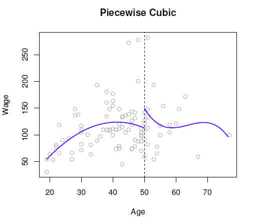
Figure 10.1: Unconstrained piecewise cubic polynomials are fit to a subset of the Wage data.
How do we fix this? The answer is to use constraints again!
The two polynomials in the above plot are of the following form. \[ \mathrm{wage} = \begin{cases} f_1({\mathrm{age}})= \beta_{01} + \beta_{11} {\mathrm{age}}+ \beta_{21} {\mathrm{age}^2}+ \beta_{31} {\mathrm{age}^3}, \,\, \mbox{if} \,\, {\mathrm{age}} < 50,\\ f_2({\mathrm{age}})= \beta_{02} + \beta_{12} {\mathrm{age}}+ \beta_{22} {\mathrm{age}^2}+ \beta_{32}{\mathrm{age}^3}, \,\, \mbox{if} \,\, {\mathrm{age}} \ge 50, \end{cases} \] We can make these two cubic polynomial lines meet at \(\mathrm{age} = 50\) by imposing the constraint \[ \beta_{01} + \beta_{11} {\mathrm{50}}+ \beta_{21} {\mathrm{50}^2}+ \beta_{31} {\mathrm{50}^3} = \beta_{02} + \beta_{12} {\mathrm{50}}+ \beta_{22} {\mathrm{50}^2}+ \beta_{32} {\mathrm{50}^3}\]
Where we can see this as a constraint on a single parameter, since, by rearranging, we get \[ \beta_{01} = \beta_{02} + (\beta_{12} - \beta_{11}) {\mathrm{50}}+ (\beta_{22}-\beta_{21}) {\mathrm{50}^2}+ (\beta_{32}-\beta_{31}) {\mathrm{50}^3} \] In other words, if we have estimates for \(\hat{\beta}_{11}\), \(\hat{\beta}_{21}\), \(\hat{\beta}_{31}\), \(\hat{\beta}_{02}\), \(\hat{\beta}_{12}\), \(\hat{\beta}_{22}\) and \(\hat{\beta}_{32}\), then \(\hat{\beta}_{01}\) is defined by the constraint.
This constraint leads to the continuous piecewise cubic polynomial seen in Figure 10.2.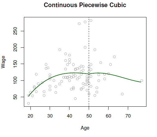
Figure 10.2: Constrained piecewise cubic polynomials are fit to a subset of the Wage data.
This looks better, although the small dip at age = 50 doesn’t make it perfect.
We therefore extend further the strategy based on constraints.
- So far we have set \(f_1(\mathrm{age = 50}) = f_2(\mathrm{age = 50})\), which ensures continuity.
- We can do the same for the first derivative: \(f^{'}_1(\mathrm{age = 50})= f^{'}_2(\mathrm{age = 50})\). This will constrain an additional parameter (coefficient), but it will make the function smoother at \(\mathrm{age = 50}\).
- Doing the same for the second derivative: \(f^{''}_1(\mathrm{age = 50})= f^{''}_2(\mathrm{age = 50})\), will constrain one more parameter, and the function will become very smooth at \(\mathrm{age = 50}\).
Can we add a further constraint on the third derivative? No, our function is cubic so the 3rd derivative is a constant (it is not a function of \(\mathrm{age}\)).
A cubic piecewise polynomial with these three constraints is called a cubic spline.
We fit a cubic spline in Figure 10.3,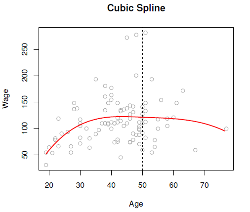
Figure 10.3: A cubic spline is fit to a subset of the Wage data.
Cubic splines are so popular because they look perfectly smooth to the human eyes! At least that is the claim…
Constraints and Degrees of Freedom
- In the previous example, we started with a cubic piecewise polynomial with 8 unconstrained parameters, so we started with 8 degrees of freedom (df).
- We initially imposed one constraint, which restricted one parameter, so we lost a degree of freedom \(\rightarrow\) 8 - 1 = 7 df.
- With the further two constraints: 8 - 3 = 5 df.
In general, a cubic spline with \(K\) knots has \(4 + K\) degrees of freedom. This is useful to know because as we will see in RStudio we can specify either the number of knots \(K\) or just the degrees of freedom.
General Definition
A degree-\(d\) regression spline is a piecewise degree-\(d\) polynomial with continuity in derivatives up to degree \(d-1\) at each knot.
The degrees of freedom of a degree-\(d\) spline with \(K\) knots are \((d+1) + K\).
- Linear spline: just continuous (2+\(K\) df)
- Quadratic spline: continuous and continuous 1st derivative (3+\(K\) df)
- Cubic spline: continuous and continuous 1st and 2nd derivatives (4+\(K\) df)
- And so on…
In general, regression splines give us the maximum amount of continuity we can have given the degree \(d\).
Spline Basis Representation
A degree-\(d\) spline with knots at \(\xi_k\) for \(k = 1,\ldots,K\) can be represented by truncated power basis functions, denoted by \(b_i\) for \(i=1,\ldots,K+d\), so that:
\[
y = \beta_0 + \beta_1 b_1(x) + \ldots + \beta_{K+d} b_{K+d}(x) + \epsilon.
\]
where:
\[\begin{align*}
b_1(x) & = x^1\\
&\vdots\\
b_d(x) &= x^d\\
b_{(k+d)}(x)& = (x - \xi_k)^d_+, ~ k = 1,\ldots, K,
\end{align*}\]
where
\[
(x - \xi_k)^d_+ = \begin{cases}
(x - \xi_k)^d~ ~ \mbox{if} \,\, x > \xi_k\\
~~~~~ 0 ~~~~~~~~ \mbox{otherwise}.
\end{cases}
\]
Example: linear spline, one knot
In the illustration shown in Figure 10.4, we just have \(y = \begin{cases} \beta_1 x, \qquad \qquad \qquad \quad \mbox{if} \,\, x<\mathrm{knot}\\ \beta_1 x + \beta_2(x - \mathrm{knot}), \,\, \mbox{if} \,\, x\ge \mathrm{knot}. \end{cases}\)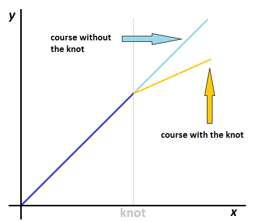
Figure 10.4: An illustration of a linear spline with a single knot.
See the recommended literature for further detail on the spline basis representation.
Example: Wage Data
In Figure 10.5, we fit a linear, quadratic and cubic spline with three knots (at the dotted lines) to a subset of the Wage data.
## Warning in if (se.fit) list(fit = predictor, se.fit = se, df = df,
## residual.scale = sqrt(res.var)) else predictor: the condition has length > 1 and
## only the first element will be used

## Warning in if (se.fit) list(fit = predictor, se.fit = se, df = df,
## residual.scale = sqrt(res.var)) else predictor: the condition has length > 1 and
## only the first element will be used

## Warning in if (se.fit) list(fit = predictor, se.fit = se, df = df,
## residual.scale = sqrt(res.var)) else predictor: the condition has length > 1 and
## only the first element will be used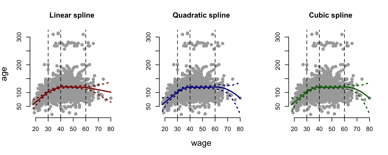
Figure 10.5: A linear, quadratic and cubic spline with three knots fit to a subset of the Wage data.
10.2 Practical Demonstration
We will continue analysing the Boston dataset included in library MASS.
Initial steps
We load library MASS again. As previously, we will analyse medv with respect to the predictor lstat. Once again, for convenience, we will name the response y and the predictor x, and pre-define plot axis labels.
library(MASS)
y = Boston$medv
x = Boston$lstat
y.lab = 'Median Property Value'
x.lab = 'Lower Status (%)'
plot(x, y, cex.lab = 1.1, col="darkgrey", xlab = x.lab, ylab = y.lab,
     main = "", bty = 'l')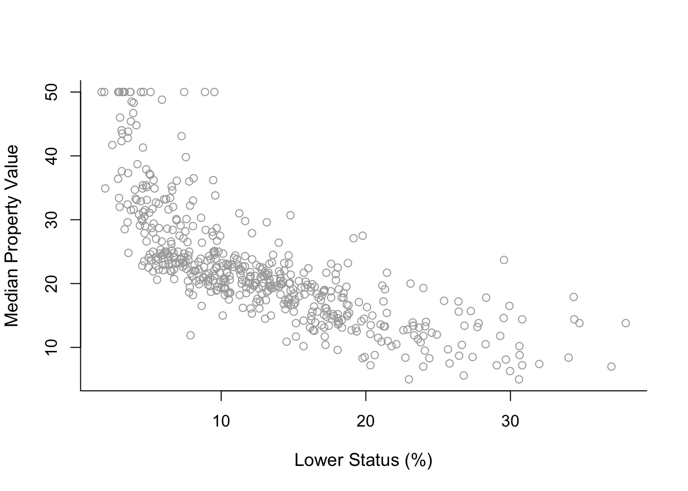
Regression Splines
For this analysis we will require package splines.
library(splines)Initially let’s fit regression splines by specifying knots. From the previous plot it is not clear where exactly we should place knots, so we will make use of the command summary in order to find the 25th, 50th and 75th percentiles of x, which will be the positions where we will place the knots.
summary(x)## Min. 1st Qu. Median Mean 3rd Qu. Max.
## 1.73 6.95 11.36 12.65 16.95 37.97cuts = summary(x)[c(2, 3, 5)]
cuts## 1st Qu. Median 3rd Qu.
## 6.950 11.360 16.955Also, before we fit the splines it is again important to sort the variable x.
sort.x = sort(x)For a start lets fit a linear spline using our selected placement of knots. For this we can use command lm() and inside it we use the command bs() in which we specify degree = 1 for a linear spline and knots = cuts for the placement of the knots at the three percentiles. We also calculate the corresponding fitted values and confidence intervals exactly in the same way we did in previous practical demonstrations.
spline1 = lm(y ~ bs(x, degree = 1, knots = cuts))
pred1 = predict(spline1, newdata = list(x = sort.x), se = TRUE)
se.bands1 = cbind(pred1$fit + 2 * pred1$se.fit,
                  pred1$fit - 2 * pred1$se.fit)
Having done that we can now produce the corresponding plot.
plot(x, y, cex.lab = 1.1, col="darkgrey", xlab = x.lab, ylab = y.lab,
     main = "Linear Spline", bty = 'l')
lines(sort.x, pred1$fit, lwd = 2, col = "red")
matlines(sort.x, se.bands1, lwd = 2, col = "red", lty = 3)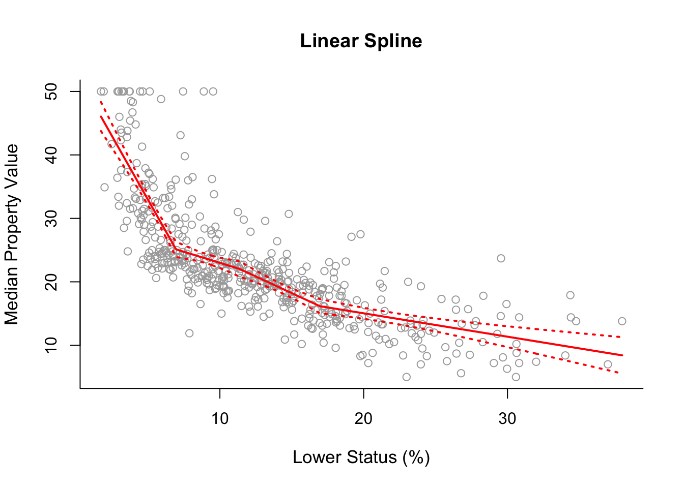
Using ?bs we see that instead of using the argument knots we can use the argument df, which are the degrees of freedom. We know that splines have \((d+1) + K\) degrees of freedom, where \(d\) is the degree of the polynomial. So in this case we have 1+1+3 = 5 degrees of freedom. Selecting df = 5 in bs() will automatically use 3 knots placed at the 25th, 50th and 75th percentiles. Below we check whether the plot based on df=5 is indeed the same as the previous plot and as we can see it is.
spline1df = lm(y ~ bs(x, degree = 1, df = 5))
pred1df = predict(spline1df, newdata = list(x = sort.x), se = TRUE)
se.bands1df = cbind( pred1df$fit + 2 * pred1df$se.fit,
                     pred1df$fit - 2 * pred1df$se.fit )

par(mfrow = c(1, 2))
plot(x, y, cex.lab = 1.1, col="darkgrey", xlab = x.lab, ylab = y.lab,
     main = "Linear Spline (with knots)", bty = 'l')
lines(sort.x, pred1$fit, lwd = 2, col = "red")
matlines(sort.x, se.bands1, lwd = 2, col = "red", lty = 3)

plot(x, y, cex.lab = 1.1, col="darkgrey", xlab = x.lab, ylab = y.lab,
     main = "Linear Spline (with df)", bty = 'l')
lines(sort.x, pred1df$fit, lwd = 2, col = "darkred")
matlines(sort.x, se.bands1df, lwd = 2, col = "red", lty = 3)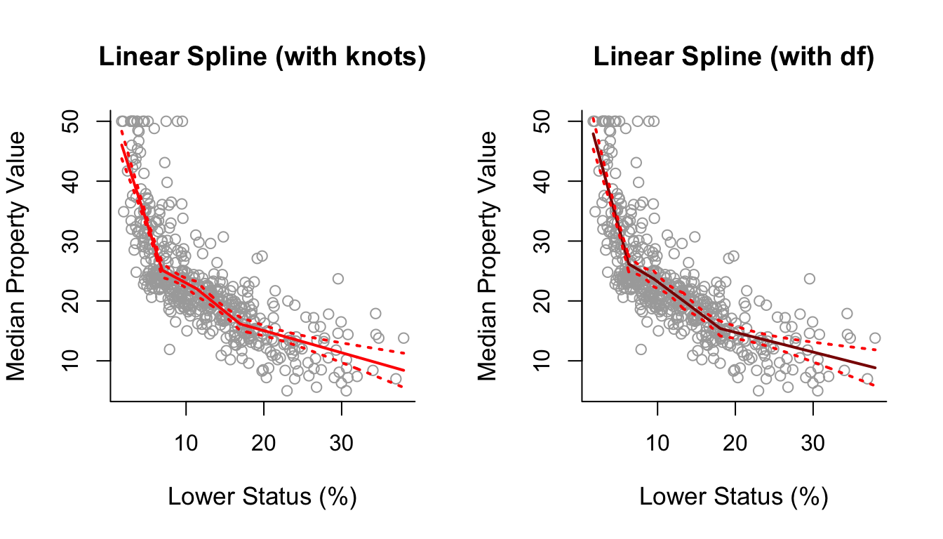
Having seen how this works we can also fit a degree-2 (quadratic) and degree-3 (cubic) spline to the data, all we have to do is change degree = 1 to degree = 2 and degree = 3 respectively. Also we increase the respective degrees of freedom from df = 5 to df = 6 and df = 7 in order to keep the same number (and position) of knots in the quadratic and cubic spline models.
spline2 = lm(y ~ bs(x, degree = 2, df = 6))
pred2 = predict(spline2, newdata = list(x = sort.x), se = TRUE)
se.bands2 = cbind(pred2$fit + 2 * pred2$se.fit, pred2$fit - 2 * pred2$se.fit)

spline3 = lm(y ~ bs(x, degree = 3, df = 7))
pred3 = predict(spline3, newdata = list(x = sort.x), se = TRUE)
se.bands3 = cbind(pred3$fit + 2 * pred3$se.fit, pred3$fit - 2 * pred3$se.fit)

par(mfrow = c(1,3))
plot(x, y, cex.lab = 1.1, col="darkgrey", xlab = x.lab, ylab = y.lab,
     main = "Linear Spline", bty = 'l')
lines(sort.x, pred1$fit, lwd = 2, col = "darkred")
matlines(sort.x, se.bands1, lwd = 2, col = "darkred", lty = 3)

plot(x, y, cex.lab = 1.1, col="darkgrey", xlab = x.lab, ylab = y.lab,
     main = "Quadratic Spline", bty = 'l')
lines(sort.x, pred2$fit, lwd = 2, col = "darkgreen")
matlines(sort.x, se.bands2, lwd = 2, col = "darkgreen", lty = 3)

plot(x, y, cex.lab = 1.1, col="darkgrey", xlab = x.lab, ylab = y.lab,
     main = "Cubic Spline", bty = 'l')
lines(sort.x, pred3$fit, lwd = 2, col = "darkblue")
matlines(sort.x, se.bands3, lwd = 2, col = "darkblue", lty = 3)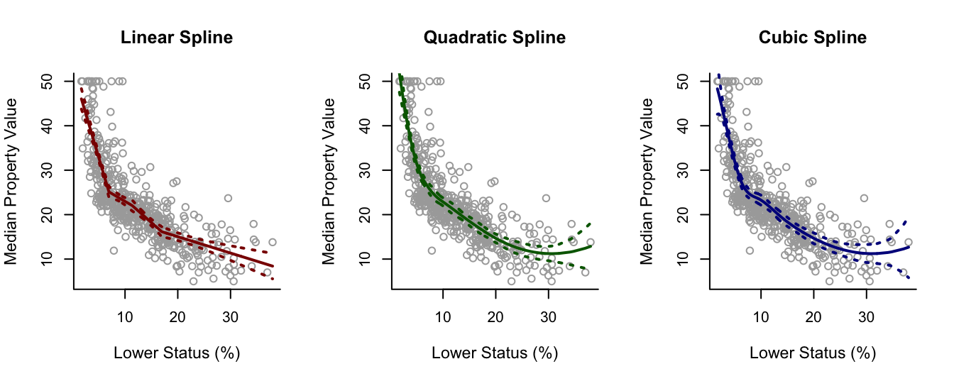
10.3 Natural Splines
Splines, especially cubic splines, seem to be the best tool we have so far, right?
Well, there is always room for improvement:
- Regression splines usually have high variance at the outer range of the predictor (the tails).
- Sometimes the confidence intervals at the tails are wiggly (especially for small sample sizes).
Natural splines are extensions of regression splines which remedy these problems to some extent.
Additional Constraints
Natural splines impose two additional constraints at each boundary region:
- The spline function is constrained to be close to linear when \(X <\) smallest knot (\(c_1\)) by \(f_0''(c_1)=0\).
- The spline function is constrained to be close to linear when \(X >\) largest knot (\(c_n\)) by \(f_n''(c_n)=0\).
These additional constraints of natural splines generally result in more stable estimates at the boundaries.
Example: Wage Data
We can see from Figure 10.6 that use of a natural spline has constrained the model at the lower and upper ends, and reduced the variance.
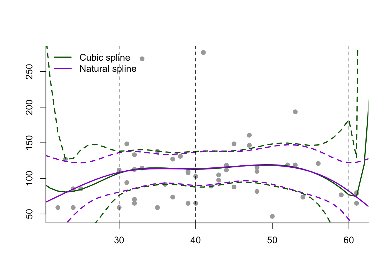
Figure 10.6: Fitting cubic and natural splines to a subset of the Wage data.
How Many Knots and Where?
- Provided there is evidence from the data we can do it empirically:
- Place knots where it is clearly obvious that we have a distributional shift in direction.
- Place more knots on regions where we see more variability.
- Place fewer knots in places which look more stable.
- Alternatively, we can place knots in a uniform fashion (e.g. at the 25th, 50th and 75th percentiles, as we saw how to do in Section 10.2).
10.4 Practical Demonstration
For natural splines, we can use the command ns() in RStudio. As with the command bs() previously, we again have the option to either specify the knots manually (via the argument knots) or to simply pre-define the degrees of freedom (via the argument df). Below we use the latter option to fit four natural splines with 1, 2, 3 and 4 degrees of freedom. As we see using 1 degree of freedom actually results in just a linear model.
spline.ns1 = lm(y ~ ns(x, df = 1))
pred.ns1 = predict(spline.ns1, newdata = list(x = sort.x), se = TRUE)
se.bands.ns1 = cbind(pred.ns1$fit + 2 * pred.ns1$se.fit,
                     pred.ns1$fit - 2 * pred.ns1$se.fit)

spline.ns2 = lm(y ~ ns(x, df = 2))
pred.ns2 = predict(spline.ns2, newdata = list(x = sort.x), se = TRUE)
se.bands.ns2 = cbind(pred.ns2$fit + 2 * pred.ns2$se.fit,
                     pred.ns2$fit - 2 * pred.ns2$se.fit)

spline.ns3 = lm(y ~ ns(x, df = 3))
pred.ns3 = predict(spline.ns3, newdata = list(x = sort.x), se = TRUE)
se.bands.ns3 = cbind(pred.ns3$fit + 2 * pred.ns3$se.fit,
                     pred.ns3$fit - 2 * pred.ns3$se.fit)

spline.ns4 = lm(y ~ ns(x, df = 4))
pred.ns4 = predict(spline.ns4, newdata = list(x = sort.x), se = TRUE)
se.bands.ns4 = cbind(pred.ns4$fit + 2 * pred.ns4$se.fit,
                     pred.ns4$fit - 2 * pred.ns4$se.fit)

par(mfrow = c(2, 2))

plot(x, y, cex.lab = 1.1, col="darkgrey", xlab = x.lab, ylab = y.lab,
     main = "Natural Spline (1 df)", bty = 'l')
lines(sort.x, pred.ns1$fit, lwd = 2, col = "darkred")
matlines(sort.x, se.bands.ns1, lwd = 2, col = "darkred", lty = 3)

plot(x, y, cex.lab = 1.1, col="darkgrey", xlab = x.lab, ylab = y.lab,
     main = "Natural Spline (2 df)", bty = 'l')
lines(sort.x, pred.ns2$fit, lwd = 2, col = "darkgreen")
matlines(sort.x, se.bands.ns2, lwd = 2, col = "darkgreen", lty = 3)

plot(x, y, cex.lab = 1.1, col="darkgrey", xlab = x.lab, ylab = y.lab,
     main = "Natural Spline (3 df)", bty = 'l')
lines(sort.x, pred.ns3$fit, lwd = 2, col = "darkblue")
matlines(sort.x, se.bands.ns3, lwd = 2, col = "darkblue", lty = 3)

plot(x, y, cex.lab = 1.1, col="darkgrey", xlab = x.lab, ylab = y.lab,
     main = "Natural Spline (4 df)", bty = 'l')
lines(sort.x, pred.ns4$fit, lwd = 2, col = "brown")
matlines(sort.x, se.bands.ns4, lwd = 2, col = "brown", lty = 3)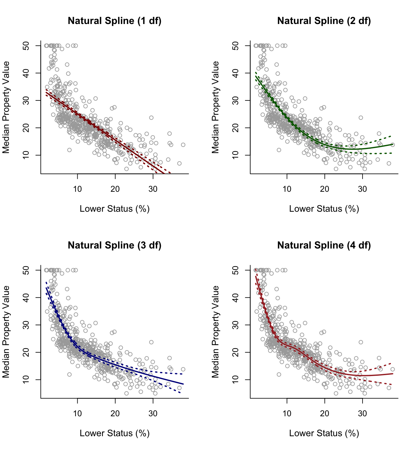
Below we plot the cubic spline next to the natural cubic spline for comparison. As we can see, the natural cubic spline is generally smoother and closer to linear on the right boundary of the predictor space, where it has, additionally, narrower confidence intervals in comparison to the cubic spline.
par(mfrow = c(1,2))
plot(x, y, cex.lab = 1.1, col="darkgrey", xlab = x.lab, ylab = y.lab,
     main = "Cubic Spline", bty = 'l')
lines(sort.x, pred3$fit, lwd = 2, col = "blue")
matlines(sort.x, se.bands3, lwd = 2, col = "blue", lty = 3)

plot(x, y, cex.lab = 1.1, col="darkgrey", xlab = x.lab, ylab = y.lab,
     main = "Natural Spline (3 df)", bty = 'l')
lines(sort.x, pred.ns3$fit, lwd = 2, col = "darkblue")
matlines(sort.x, se.bands.ns3, lwd = 2, col = "darkblue", lty = 3)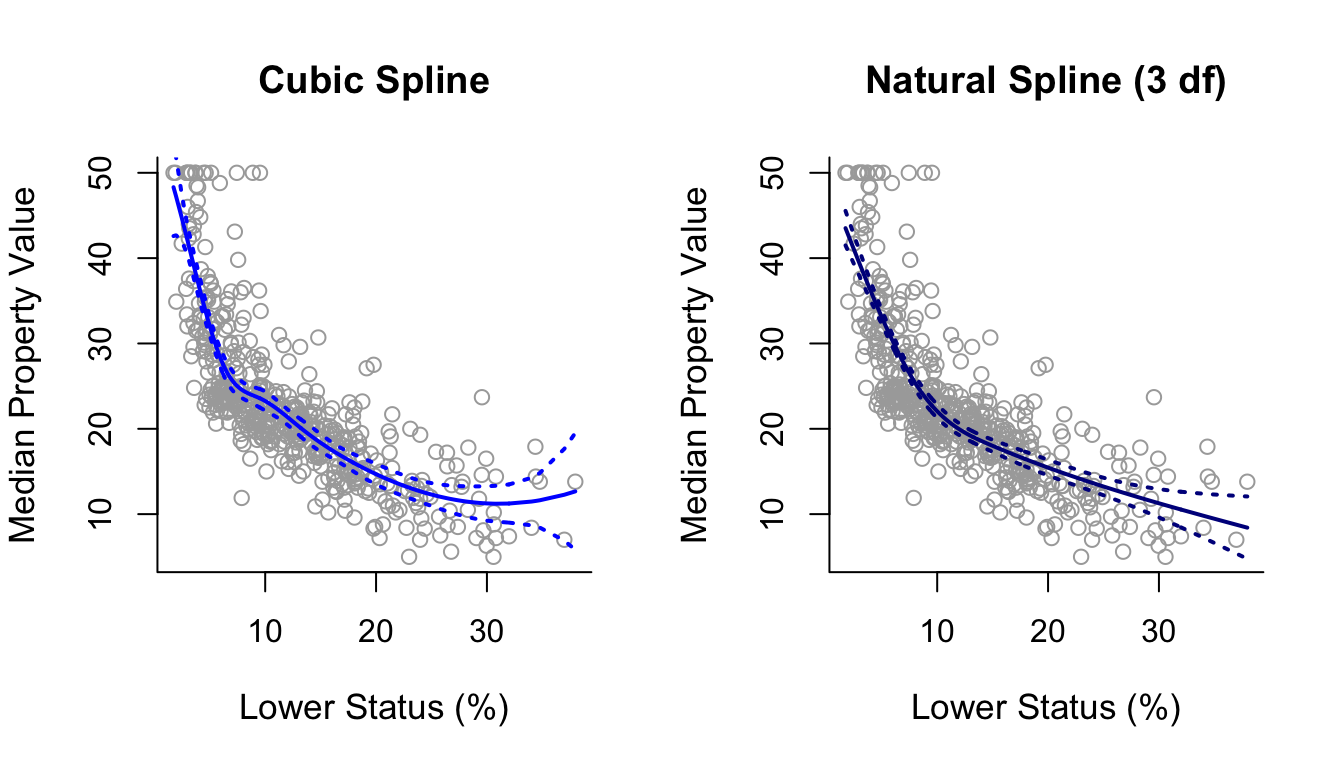
10.5 Smoothing Splines
Smoothing splines are quite different from the non-linear modelling methods we have seen so far. Unlike regression splines and natural splines, there are no knots! Smoothing splines turns the discrete problem of selecting a number of knots into a continuous penalisation problem. The maths here is rather complicated, so we mainly introduce this topic by intuition rather than go into a load of technical details.
Minimisation
We seek a function \(g\) among all possible functions (linear or non-linear) which minimises \[ \sum_{i=1}^{n}(y_i - g(x_i))^2 + \lambda \int \left({g}''(t)\right)^2\mathrm{d}t, \] where \(\lambda \ge 0\) is a tuning parameter.
The function \({g}\) that minimises the above quantity is called a smoothing spline.
Model Fit \(+\) Penalty Term
\[ \underbrace{\sum_{i=1}^{n}(y_i - g(x_i))^2}_{\mbox{Model fit}} + \underbrace{\lambda \int \left(g{''}(t)\right)^2\mathrm{d}t}_{\mbox{Penalty term}} \]
- When \(\lambda = 0\) we are just left with the model fit term.
- When \(\lambda \rightarrow \infty\)… well more on that later.
- Lets examine the two terms separately.
The Model Fit Term
\[\sum_{i=1}^{n}(y_i - g(x_i))^2\] This is a RSS but not our “usual” RSS:
- In all previous approaches, function \(g\) was linear in the parameters (coefficients of the predictors) and we minimised with respect to these parameters.
- Here, we have one predictor but the minimisation is with respect to \(g\)!
- So, if we let \(g\) be unconstrained and just minimise the above RSS, then we can end up with any weird-looking non linear function that passes through exactly every data point, leading to an RSS equal to 0 (overfitting!).
Thus, the penalty on \(g\)…
The Penalty Term
\[\lambda \int \left(g{''}(t)\right)^2\mathrm{d}t\]
- \(g''(t)\) is the 2nd derivative of \(g\) at a point \(t\) within the space of predictor \(X\).
- The 2nd derivative of a function catches wiggles or non-linearities: if \(g''(t^*)^2\) at a point \(t^*\) is large, this means that \(g\) at this point \(t^*\) suddenly jumps either up or down.
- The integration above over every \(t\) in the space of \(X\) is essentially a sum. The larger it is the more non-linear the function \(g\) is.
Putting it all Together
Minimizing \[ \sum_{i=1}^{n}(y_i - g(x_i))^2 + \lambda \int \left(g{''}(t)\right)^2\mathrm{d}t, \] with respect to \(g\) turns out to be interesting.
- When \(\lambda=0\) we get an extremely wiggly non-linear function \(g\) (completely useless).
- As \(\lambda\) increases, the function \(g\) will become smoother.
- In the theoretical case of \(\lambda \rightarrow \infty\), \(g''\) will be zero everywhere. When does that happen? When \(g(x) = \beta_0 + \beta_1x\). So, in this case we return back to the linear model!
That is why the penalty term is also called a roughness penalty within the framework of smoothing splines.
Solution
Surprisingly, the solution for any finite and non-zero \(\lambda\) is that the function \(g\) is a natural cubic spline but with knots placed on each individual sample point \(x_1, \ldots, x_n\).
But doesn’t that lead to overfitting? No, because now we have once again the penalty parameter \(\lambda\) which can shrink coefficients to zero and thus avoid overfitting.
Tuning \(\lambda\)
- As usual \(\lambda\) can be tuned via cross-validation.
- Also, \(\lambda\) is associated with the effective degrees of freedom of a smoothing spline. These are similar to the degrees of freedom in standard spline models and can be used as an alternative to cross-validation as a way to fix \(\lambda\).
10.6 Practical Demonstration
Boston Data
For fitting smoothing splines we use the command smooth.splines() instead of lm(). Under smoothing splines there are no knots to specify; the only parameter is \(\lambda\). This can be specified via cross-validation by specifying cv = TRUE inside smooth.splines(). Alternatively, we can specify the effective degrees of freedom which correspond to some value of \(\lambda\). Below we use cross-validation as well as a smoothing spline with 3 effective degrees of freedom (via the argument df = 3). In this case we see that tuning \(\lambda\) through cross-validation results in a curve which is slightly wiggly on the right boundary of the predictor space.
smooth1 = smooth.spline(x, y, df = 3)
smooth2 = smooth.spline(x, y, cv = TRUE)

par(mfrow = c(1,2))
plot(x, y, cex.lab = 1.1, col="darkgrey", xlab = x.lab, ylab = y.lab,
     main = "Smoothing Spline (3 df)", bty = 'l')
lines(smooth1, lwd = 2, col = "brown")

plot(x, y, cex.lab = 1.1, col="darkgrey", xlab = x.lab, ylab = y.lab,
     main = "Smoothing Spline (CV)", bty = 'l')
lines(smooth2, lwd = 2, col = "darkorange")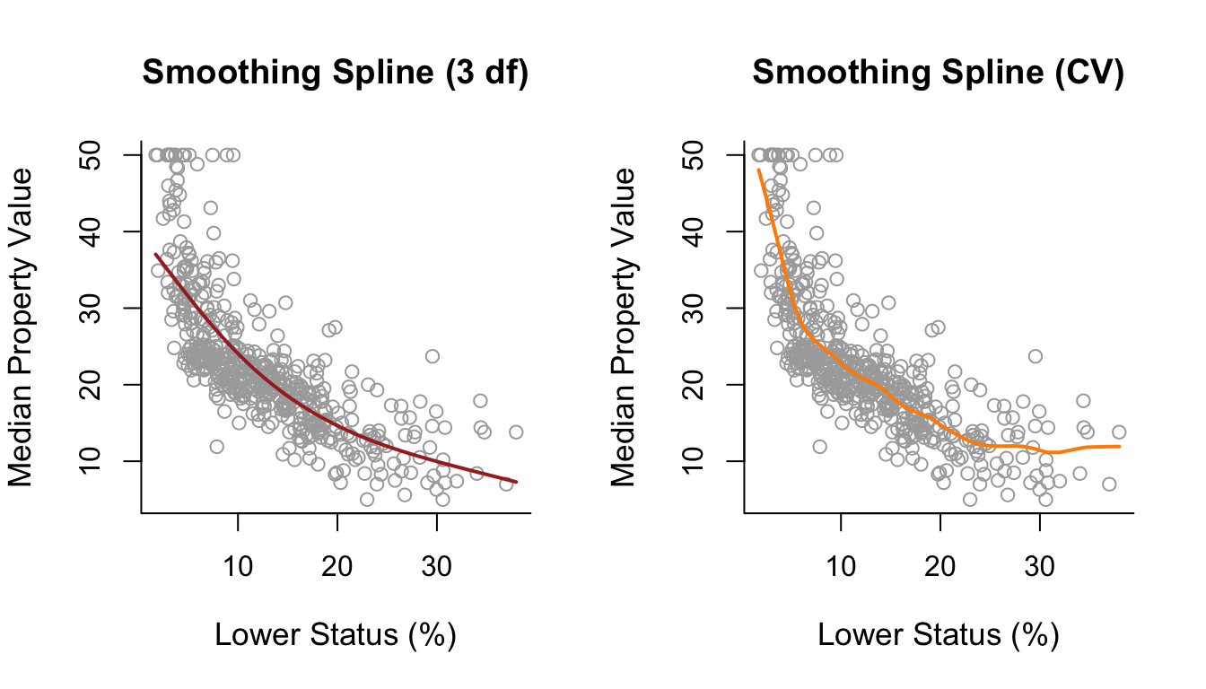
Wage Data
Lets see how cubic splines, natural cubic splines and smoothing splines compare on the Wage data.
We will take sample size into consideration and see how the fitted curves look like for:
- A small sample of 50.
- A medium sample of 200.
- A large sample of 1000.
For the cubic spline and natural cubic spline we have to define the number and position of the knots. For simplicity we will adopt the previous strategy: 3 knots placed at the ages of 30, 40 and 60.
For the smoothing spline, everything is automatic - \(\lambda\) will be determined via CV by setting cv = TRUE.
Note that the code below runs this comparison for a sample size of \(n=200\). To plot results for \(n=50\) and \(n=1000\) (or any other value of \(n\)!), run the code yourself in R and change the line n <- 200 so that n is your chosen size.
library("ISLR")
library("splines") # Required for regression and natural splines.
agelims=range(Wage$age)
age.grid=seq(from=agelims[1],to=agelims[2])

set.seed(1)

# Number of data points - change this to investigate
# small, medium and large samples.
n <- 200

# Take the a sample of n points from the data.
ind = sample(1:3000, n)
Wage1 = Wage[ind,]  # Label subset of data as Wage1.

# Cubic Spline
fitbs = lm(wage~bs(age, degree = 3, knots = c(30,40,60)), data = Wage1)
predbs = predict(fitbs, newdata = list(age = age.grid), se = T)

# Natural Spline
fitns = lm(wage~ns(age, knots = c(30,40,60)), data = Wage1)
predns = predict(fitns, newdata = list(age = age.grid), se = T)

# Smoothing Spline
fitss = smooth.spline(Wage1$age, Wage1$wage, cv = TRUE)

# Generate the Plots.
par(mfrow=c(1,3))

# Cubic Spline
plot(Wage1$age, Wage1$wage, col = "darkgray", pch = 19,
     main = 'Cubic spline', bty = 'l',
     xlab = 'age', ylab = 'wage', cex.lab = 1.4)
lines(age.grid, predbs$fit, lwd = 2, col = 'darkgreen')
abline(v = c(30,40,60), lty = 'dashed')

# Natural Spline
plot(Wage1$age, Wage1$wage, col = "darkgray", pch = 19,
     main = 'Natural cubic spline', bty = 'l',
     xlab = 'age', ylab = 'wage', cex.lab = 1.4)
lines(age.grid, predns$fit, lwd = 2, col = 'darkviolet')
abline(v = c(30,40,60), lty = 'dashed')

# Smoothing Spline
plot(Wage1$age, Wage1$wage, col = "darkgray", pch = 19,
     main = 'Smoothing spline', bty = 'l',
     xlab = 'age', ylab = 'wage', cex.lab = 1.4)
lines(fitss, lwd = 2, col = 'brown')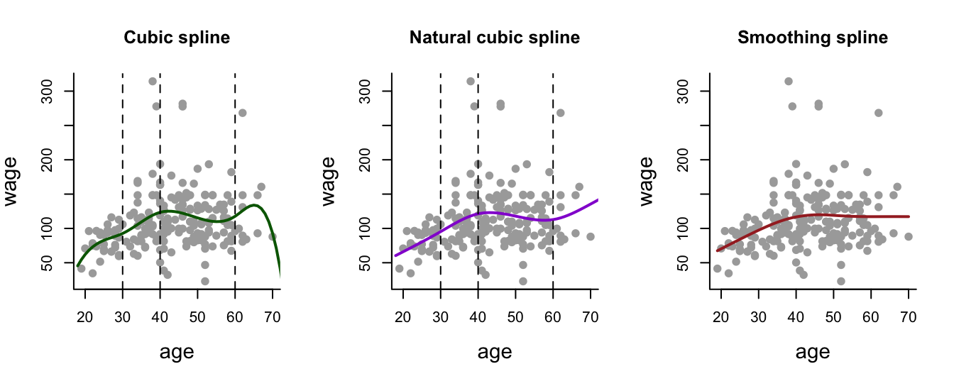
- If you run the above code for various sample sizes, you will see that, overall, the smoothing spline method is more robust: the shape of the curve remains more or less stable across different sample sizes. Importantly, this means that the fitted curve from the smoothing spline under \(n = 50\) would fit well to the data with \(n = 1000\).
- That is not the case for the other two methods, especially for the cubic spline. These methods are more sensitive to the particular sample being used to train them.
Drawback
You will notice that we didn’t plot confidence intervals, because there is no built-in function in R package smooth.splines (that we used) that produces confidence intervals for smoothing splines.
This is not a flaw of the package; this is a generic issue with smoothing splines as it is not as straightforward as it is with other spline methods to calculate confidence intervals.
One can get confidence-like intervals by using:
- Bayesian credible intervals
- Bootstrap
These methods require additional work and are beyond the scope of this course.