Practical Class Sheets 1

In this practical class, we will use R to fit linear regression models by the method of least squares (LS). We will make use of R’s lm function simplify the process of model fitting and parameter estimation, and use information from its output to construct confidence intervals. Finally, we will assess the quality of the regression and use residual diagnostic plots to assess the validity of the regression assumptions.

To start, create a new R script by clicking on the corresponding menu button (in the top left); and save it somewhere in your computer. You can now write all your code into this file, and then execute it in R using the menu button Run or by simple pressing ctrl $+$ enter.

$~$

The `faithful` data set

The dataset we will be using in this practial class concerns the behaviour of the Old Faithful geyser in Yellowstone National Park, Wyoming, USA. For a natural phenomenon, the Old Faithful geyser is highly predictable and has erupted every 44 to 125 minutes since 2000. There are two variables in the data set:

the waiting time between eruptions of the geyser, and
the duration of the eruptions.

Before we start fitting any models, the first step should always be to perform some exploratory data analysis of the data to gain some insight into the behaviour of the variables and suggest any interesting relationships or hypotheses to explore further.

Exercise 1.1

Load the faithful dataset by typing data(faithful)
To save typing later, let us extract the columns into two variables. Create a vector w that contains the vector of waiting times, and a second vector d that contains the durations of eruptions.
Plot the waiting times (y-axis) against the durations (x-axis).
Compute the Pearson correlation coefficient between w and d using the cor function.
Is there evidence of a linear relationship?

Click for solution

## SOLUTION
data(faithful)
w <- faithful$waiting
d <- faithful$eruptions
cor(w, d)

## [1] 0.9008112

plot(y=w,x=d)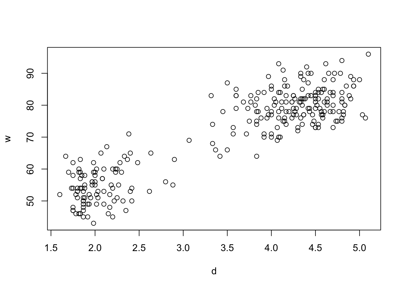

$~$

Fitting the simple linear regression model

The model we’re interested in fitting to these data is a simple linear relationship between the waiting times, $w$, and the eruption durations, $d$: \[ w = \beta_0 + \beta_1 d + \varepsilon.\]

R provides the lm function to compute the least-squares linear regression for us, and it returns an object which summarises all aspects of the regression fit.

Technique

In R, we can fit linear models by the method of least squares using the function lm. Suppose our response variable is $Y$, and we have a predictor variable $X$, with observations stored in R vectors y and x respectively. To fit $y$ as a linear function of $x$, we use the following lm command:

model <- lm(y ~ x)

Alternatively, if we have a data frame called dataset with variables in columns a and b then we could fit the linear regression of a on b without having to extract the columns into vectors by specifying the data argument

model <- lm(a ~ b, data=dataset)

The ~ (tilde) symbol in this expression should be read as “is modelled as”. Note that R always automatically include a constant term, so we only need to specify the $X$ and $Y$ variables.

We can inspect the fitted regression object returned from lm to get a simple summary of the estimated model parameters. To do this, simply evaluate the variable which contains the information returned from lm: model

Exercise 1.2

Use lm to fit waiting times w as a linear function of eruption durations d.
Save the result of the regression function to model.
Inspect the value of model to find the fitted least-squares coefficients.

Click for solution

## SOLUTION
# lm(y ~ x) use only x variable 
# lm(y ~ .) use all predictors
# lm(y ~ 1) intercept only

model <- lm(w~d)
model

## 
## Call:
## lm(formula = w ~ d)
## 
## Coefficients:
## (Intercept)            d  
##       33.47        10.73

\[ \]

Technique

R also has a number of functions that, when applied to the results of a linear regression, will return key quantities such as residuals and fitted values.

coef(model) and coefficicents(model) – returns the estimated model coefficients as a vector $(b_0,b_1)$
fitted(model) and fitted.values(model) – returns the vector of fitted values, $\widehat{y}_i=b_0+b_1 x_i$
resid(model) and residuals(model) – returns the vector of residual values, $e_i=y_i-\widehat{y}_i$

Exercise 1.3

Use the coef function to extract the coefficients of the fitted linear regression model as a vector.
Extract the vector of residuals from model, and use this to compute the sum of squares of the residuals as lsq.Q.

Click for solution

## SOLUTION
# (a)
coef(model)

## (Intercept)           d 
##    33.47440    10.72964

beta0hat <- coef(model)[1]
beta0hat

## (Intercept) 
##     33.4744

beta1hat <- coef(model)[2]
beta1hat

##        d 
## 10.72964

# (b)
lsq.resid <- resid(model)
lsq.Q <- sum(lsq.resid^2)
lsq.Q

## [1] 9443.387

$~$

The regression summary

Technique

We can easily extract and inspect the coefficients and residuals of the linear model, but to obtain a more complete statistical summary of the model we use the summary function.:

summary(model)

There is a lot of information in this output, but the key quantities to focus on are:

Residuals: simple summary statistics of the residuals from the regression.
Coefficients: a table of information about the fitted coefficients. Its columns are:
- The label of the fitted coefficient: The first will usually be (Intercept), and subsequent rows will be named after the other predictor variables in the model.
- The Estimate column gives the least squares estimates of the coefficients.
- The Std. Error column gives the corresponding standard error for each coefficient.
- The t value column contains the $t$ test statistics.
- The Pr(>|t|) column is then the $p$-value associated with each test, where a low p-value indicates that we have evidence to reject the null hypothesis.
Residual standard error: This gives ${s_e}$ the square root of the unbiased estimate of the residual variance.
Multiple R-Squared: This is the $R^2$ value defined in lectures as the squared correlation coefficient and is a measure of goodness of fit.

We can also use the summary to access the individual elements of the regression summary output. If we save the results of a call to the summary function of a lm object as summ:

summ$residuals – extracts the regression residuals as resid above
summ$coefficients – returns the $p \times 4$ coefficient summary table with columns for the estimated coefficient, its standard error, t-statistic and corresponding (two-sided) p-value.
summ$sigma – extracts the regression standard error
summ$r.squared – returns the regression $R^2$

Exercise 1.4

Apply the summary function to model to produce the regression summary for our example.
Make sure you are able to locate:
- The coefficient estimates, and their standard errors,
- The residual standard error, ${s_e}$;
- The regression $R^2$.
Extract the regression standard error from the regression summary, and save it as se. (We’ll need this later!)
What do the entries in the t value column correspond to? What significance test (and what hypotheses) do these statistics correspond to?
Are the coefficients significant or not? What does this suggest about the regression?
What is the $R^2$ value for the regression and what is its interpretation? Can you extract its numerical value from the output as a new variable?
Does the $R^2$ value ‘agree’ with the Pearson correlation coefficient between w and d you calculated early.

Click for solution

## SOLUTION
# (a) & (b)
summary(model)

## 
## Call:
## lm(formula = w ~ d)
## 
## Residuals:
##      Min       1Q   Median       3Q      Max 
## -12.0796  -4.4831   0.2122   3.9246  15.9719 
## 
## Coefficients:
##             Estimate Std. Error t value            Pr(>|t|)    
## (Intercept)  33.4744     1.1549   28.98 <0.0000000000000002 ***
## d            10.7296     0.3148   34.09 <0.0000000000000002 ***
## ---
## Signif. codes:  0 '***' 0.001 '**' 0.01 '*' 0.05 '.' 0.1 ' ' 1
## 
## Residual standard error: 5.914 on 270 degrees of freedom
## Multiple R-squared:  0.8115, Adjusted R-squared:  0.8108 
## F-statistic:  1162 on 1 and 270 DF,  p-value: < 0.00000000000000022

# (c)
se <- summary(model)$sigma
se

## [1] 5.914009

# (d) & (e)
# The column t value shows you the t-test associated with testing the significance 
# of the parameter listed in the first column. 
# Both coefficients are significant, as p-values are very small.

# (f)
rsq <- summary(model)$r.squared
rsq

## [1] 0.8114608

# (g)
cor(w, d)^2

## [1] 0.8114608

$~$

Inference on the coefficicents

Given a fitted regression model, we can perform various hypothesis tests and construct confidence intervals to perform the usual kinds of statistical inference. To do this, we require the Normality assumption to hold for our inference to be valid.

Theory tells us that the standard errors for the parameter estimates are defined as \[ s_{b_0} = s_e \sqrt{\frac{1}{n}+\frac{\bar{x}^2}{S_{xx}}}, ~~~~~~~~~~~~~~~~~~~~ s_{b_1} = \frac{s_e}{\sqrt{S_{xx}}}, \] where $s_{b_0}$ and $s_{b_1}$ are unbiased estimates for $\sigma_{b_0}$ and $\sigma_{b_0}$, the variances of $b_0$ and $b_1$.

Given these standard errors and the assumption of normality, we can say for coefficient $\beta_i$, $i=0,1$ that: \[ \frac{b_i - \beta_i}{s_{b_i}} \sim \mathcal{t}_{{n-2}}, \] and hence an $\alpha$ level confidence interval for $\beta_i$ can be written as \[ b_i \pm t^*_{n-2,\alpha/2} ~ s_{b_i}. \]

Exercise 1.5

Consider the regression slope. Use the regression summary to extract the standard error of $b_1$. Assign its value to the variable se.beta1.
Compute the test statistic defined above using beta1hat and se.beta1 for a test under the null hypothesis $H_0: \beta_1=0$. Does it agree with the summary output from R?
Use the pt function to find the probability of observing a test statistic as extreme as this.
Referring to your $t$-test statistic and the t values in the regression summary, what do you conclude about the significance of the regression coefficients?
Find a 95% confidence interval for the slope $\beta_1$. You’ll need to use the qt function to find the critical value of the $t$-distribution.
An easy way to find the confidence interval in (e) is by using the function confint.

Click for solution

## SOLUTION
# (a)
# extract the standard error from the second column of the coefficient summary table
se.beta1 <- summary(model)$coefficients[2,2]
se.beta1

## [1] 0.3147534

# (b)
## compute the t statistic
t.beta1 <- (beta1hat-0)/se.beta1
t.beta1

##        d 
## 34.08904

t.beta1<-unname(t.beta1)
t.beta1

## [1] 34.08904

# (c)
## p-value
n <- length(w)
2*(1-pt(t.beta1, n-2)) # df =n-2

## [1] 0

# (e)
## confidence interval
beta1hat + c(-1,1) * qt(0.975,n-2) * se.beta1

## [1] 10.10996 11.34932

# (f)
confint(model, level = 0.95)

##                2.5 %   97.5 %
## (Intercept) 31.20069 35.74810
## d           10.10996 11.34932

# for the slope parameter
confint(model, parm = "d", level = 0.95)

##      2.5 %   97.5 %
## d 10.10996 11.34932

# or
confint(model, level = 0.95)[2,]

##    2.5 %   97.5 % 
## 10.10996 11.34932

$~$

Estimation and prediction

Suppose now that we are interested in some new point $X=x^*$, and at this point we want to predict: (a) the location of the regression line, and (b) the value of $Y$.

In the first problem, we are interested in the value $\mu^*=\beta_0+\beta_1 x^*$, i.e. the location of the regression line, at some new point $X=x^*$.

In the second problem, we are interested in the value of $Y^*=\beta_0+\beta_1 x^*+\varepsilon$, i.e. the actual observation value, at some new $X=x^*$.

The difference between the two is that the first simply concerns the location of the regression line, whereas the inference for the new observation $Y^*$ concerns both the position of the regression line and the regression error about that point.

Exercise 1.6

Find a 95% confidence interval for the estimated waiting time $\widehat{W}$ when the eruption duration is 3 minutes using the predict function.
Find a 95% prediction interval for the actual waiting time, $W$.
Compare the two intervals.

Click for solution

## SOLUTION
newdata1<- data.frame(d = 3)
predict(model, newdata = newdata1, interval = "confidence", level = 0.95)

##        fit      lwr     upr
## 1 65.66332 64.89535 66.4313

predict(model, newdata = newdata1, interval = "prediction", level = 0.95)

##        fit      lwr      upr
## 1 65.66332 53.99458 77.33206

$~$

Residual Analysis

The residuals from our linear regression are the values $e_i=\widehat{\varepsilon_i} = y_i - \widehat{y}_i$ for $i = 1,\dots,n$, where $\widehat{y}_i=b_0-b_1 x_i$. Analysis of the residuals allow us to perform diagnostic tests to investigate the goodness of fit of our regression under our modelling assumptions.

Under the assumption of linearity, given the LS estimates, the observed values of $X$ are uncorrelated with the residuals. Which, in the case of simple linear regression, implies that the residuals are uncorrelated with any linear combination of $X$, in particular the fitted values $\widehat{y}_i=b_0+b_1 x_i$. Therefore, our diagnostics are based on the scatterplots of $e$ against $\widehat{y}$. In the case of simply linear regression will look the same as plotting $e$ against $x$.

To assess the SLR assumptions, we inspect the residual plot for particular features:

Even and random scatter of the residuals about $0$ is the expected behaviour when our SLR assumptions are satisfied.
Residuals shown evidence of a trend or pattern — The presence of a clear pattern or trend in the residuals suggests that $\mathbb{E}\left[\epsilon\right]_i\neq 0$ and $\mathbb{C}ov\left[\epsilon_i,\epsilon_j\right]\neq 0$. There is clearly structure in the data that is not explained by the regression model, and so a simple linear model is not adequate for explaining the behaviour of $Y$.
Spread of the residuals is not constant — if the spread of the residuals changes substantially as $x$ (or $\widehat{y}$) changes then clearly our assumption of constant variance is not upheld.
A small number of residuals are very far from the others and $0$ — observations with very large residuals are known as outliers. Sometimes these points can be explained through points with particularly high measurement error, or the effect of another variable which should be included in the model. Their presence could signal problems with the data, a linear regression being inadequate, or a violation of Normality.

Exercise 1.7

Plot the residuals against the fitted values, and the residuals against the eruption durations side-by-side.
What do you see? Why should these plots be similar?
Use your residual plot to assess whether the SLR assumptions are valid for these data.

Click for solution

par(mfrow=c(1,2))
plot(y=resid(model), x=fitted(model))
plot(y=resid(model), x=d)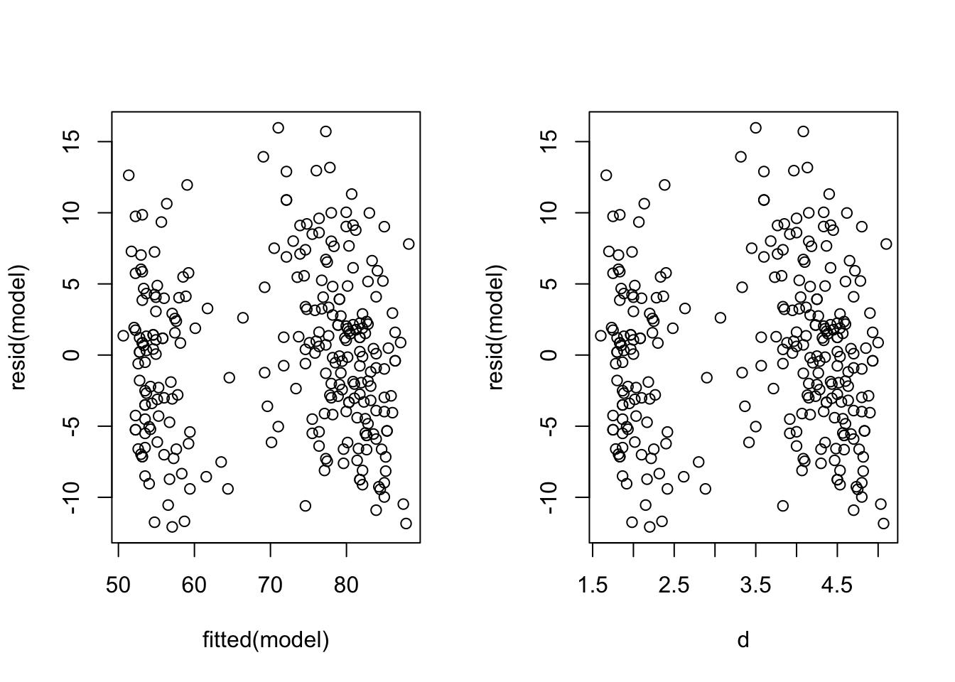

$~$

In order to state confidence intervals for the coefficients and for predictions made using this model, in addition to the assumptions tested above, we also require that the regression errors are normally distributed. We can check the normality assumption using quantile plots.

Exercise 1.8

Produce a side-by-side plot of the histogram of the residuals and a normal quantile plot of the residuals.
Do the residuals appear to be normally distributed?

Click for solution

par(mfrow=c(1,2))
hist(resid(model))
qqnorm(resid(model))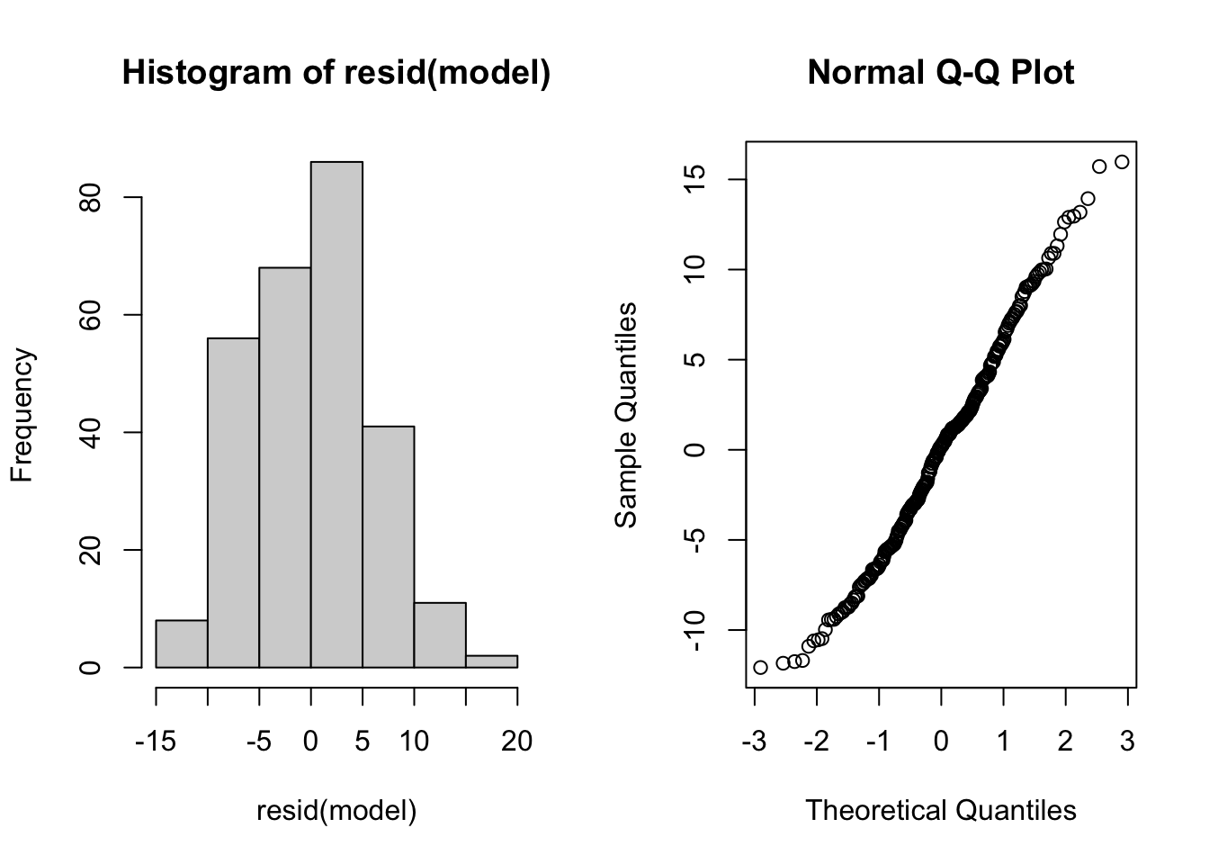

$~$

Practical Class Sheets 1

The faithful data set

Fitting the simple linear regression model

The regression summary

Inference on the coefficicents

Estimation and prediction

Residual Analysis

The `faithful` data set