Chapter 2 Definitions and Basic Concepts
2.1 Types of data
Data sets can consist of two types of data:
Qualitative (categorical) data consist of attributes, labels, or nonnumerical entries. e.g. name of cities, gender etc.
Quantitative data consist of numerical measurements or counts. e.g. heights, age, temperature. Quantitative data can be distinguished as:
Discrete data result when the number of possible values is either a finite number or a “countable” number. e.g. the number of phone calls you received on any given day.
Continuous data result from infinitely many possible values that correspond to some continuous scale that covers a range of values without gaps, interruptions, or jumps. e.g. height, weight, sales and market shares.
2.2 Supervised and Unsupervised Learning
Every machine learning task can be broken down into either supervised learning or unsupervised learning.
Supervised learning involves building a statistical model for predicting or estimating an output based on one or more inputs.
Supervised learning aims to learn a mapping \(f\) from inputs \(\bf{x}\in \mathcal{X}\) to outputs \(\bf{y}\in \mathcal{Y}\). The inputs \(\bf{x}\) are also called the features, covariates, or predictors ; this is often a fixed-dimensional vector of numbers, such as the height and weight of a person, or the pixels in an image. In this case, \(\mathcal{X} = \mathbb{R}^D\) , where \(D\) is the dimensionality of the vector (i.e., the number of input features). The output \(\bf{y}\) is also known as the label , target, or response. In supervised learning, we assume that each input example \(\bf{x}\) in the training archive has an associated set of output targets \(\bf{y}\), and our goal is to learn the input-output mapping \(f\).
The task of Unsupervised learning is to try to “make sense of” data, as opposed to just learning a mapping. That is, we just get observed “inputs” \(\bf{x}\in \mathcal{X}\) without any corresponding “outputs” \(\bf{y}\in \mathcal{Y}\).
From a probabilistic perspective, we can view the task of unsupervised learning as fitting an unconditional model of the form \(p(\bf{x})\), which can generate new data \(\bf{x}\), whereas supervised learning involves fitting a conditional model, \(p(\bf{y}|\bf{x})\), which specifies (a distribution over) outputs given inputs.
Unsupervised learning avoids the need to collect large labelled datasets for training, which can often be time-consuming and expensive (think of asking doctors to label medical images). Unsupervised learning also avoids the need to learn how to partition the world into often arbitrary categories. Finally, unsupervised learning forces the model to “explain” the high-dimensional inputs, rather than just the low-dimensional outputs. This allows us to learn richer models of “how the world works” and discover “interesting structure” in the data.
Here is a simple example that shows the difference between supervised learning and unsupervised learning.
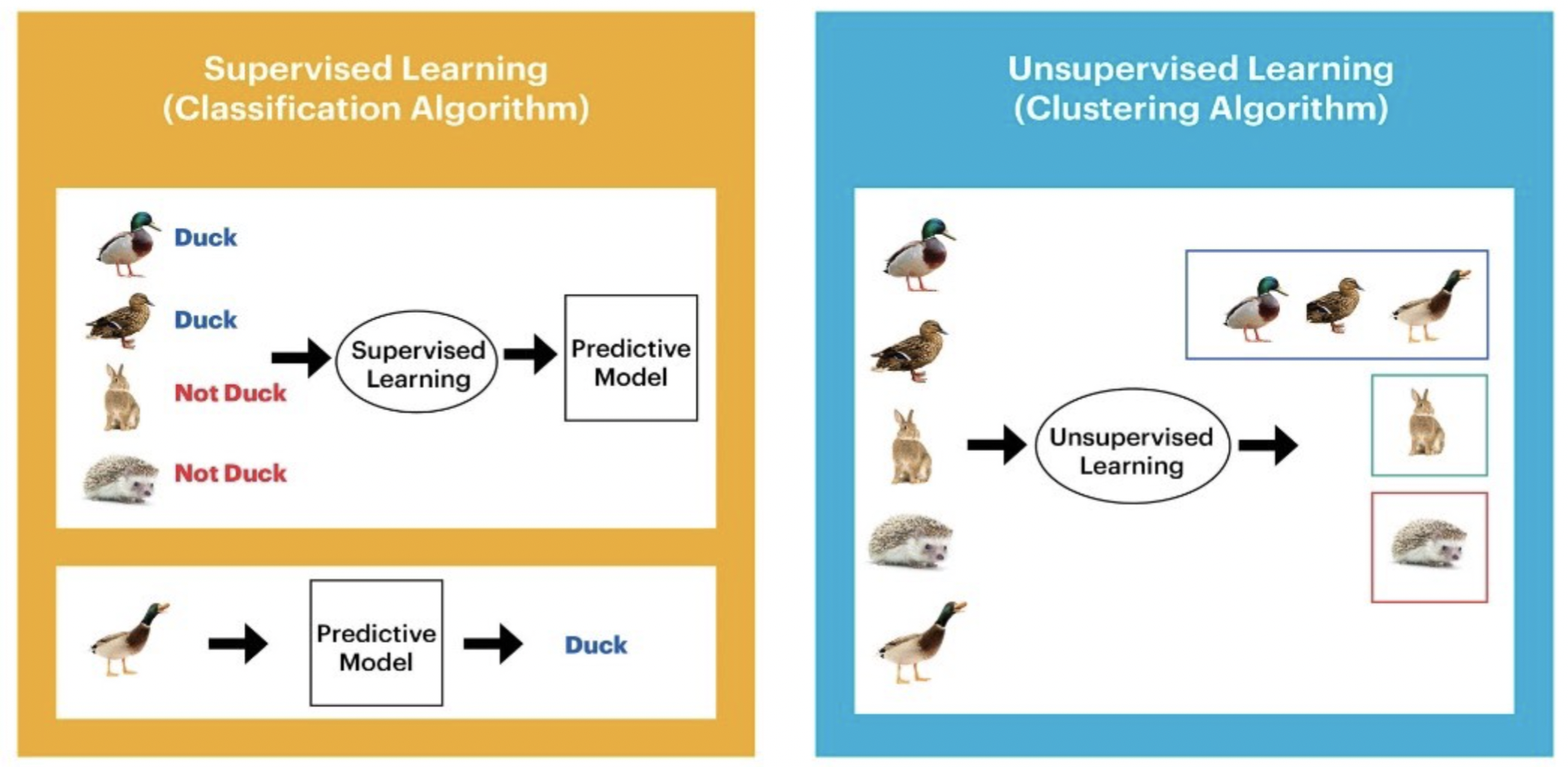
Many classical machine (statistical) learning methods such as linear regression and logistic regression as well as more advanced approaches such as random forests and boosting operate in the supervised learning domain. Most part of this course will be devoted to this setting. For unsupervised learning, we will cover one of the classic linear approaches, principal component analysis, in the first term of the course.
2.3 Classification and Regression
Supervised learning can be further divided into two types of problems: Classification and Regression.
Classification
Classification algorithms are used when the output variable is categorical
The task of the classification algorithm is to find the mapping function to map the input(\(\bf{x}\)) to the discrete output(\(\bf{y}\)).
Example: The best example to understand the Classification problem is Email Spam Detection. The model is trained on the basis of millions of emails on different parameters, and whenever it receives a new email, it identifies whether the email is spam or not. If the email is spam, then it is moved to the Spam folder.
Regression
Regression algorithms are used if there is a relationship between the input variable and the output variable. It is used for the prediction of continuous variables, such as Weather forecasting, Market Trends, etc.
Regression is a process of finding the correlations between dependent and independent variables. It helps in predicting the continuous variables such as prediction of Market Trends, prediction of House prices, etc.
The task of the Regression algorithm is to find the mapping function to map the input variable(x) to the continuous output variable(y).
Example: Suppose we want to do weather forecasting, so for this, we will use the Regression algorithm. In weather prediction, the model is trained on the past data, and once the training is completed, it can easily predict the weather for future days.
2.4 Parametric vs non-parametric models
Machine learning models can be parametric or non-parametric. Parametric models are those that require the specification of some parameters, while non-parametric models do not rely on any specific parameter settings.
Parametric models
Assumptions about the form of a function can ease the process of machine learning. Parametric models are characterized by the simplification of the function to a known form. A parametric model is a learner that summarizes data through a collection of parameters, \(\bf{\theta}\). These parameters are of a fixed size. This means that the model already knows the number of parameters it requires, regardless of its data.
As an example, let’s look at a simple linear regression model (we will investigate this model thoroughly in the following chapter) in the functional form: \[y=b_0+b_1x+\epsilon\] where \(b_0\) and \(b_1\) are model parameters and \(\epsilon\) reflects the model error. For such a model, feeding in more data will impact the value of the parameters in the equation above. It will not increase the complexity of the model. And note this model form assumes a linear relationship between the input \(x\) and response \(y\).
Non-parametric models
Non-parametric models do not make particular assumptions about the kind of mapping function and do not have a specific form of the mapping function. Therefore they have the freedom to choose any functional form from the training data.
One might think that non-parametric means that there are no parameters. However, this is NOT true. Rather, it simply means that the parameters are (not only) adjustable but can also change. This leads to a key distinction between parametric and non-parametric algorithms. We mentioned that parametric algorithms have a fixed number of parameters, regardless of the amount of training data. However, in the case of non-parametric ones, the number of parameters is dependent on the amount of training data. Usually, the more training data, the greater the number of parameters. A consequence of this is that non-parametric models may take much longer to train.
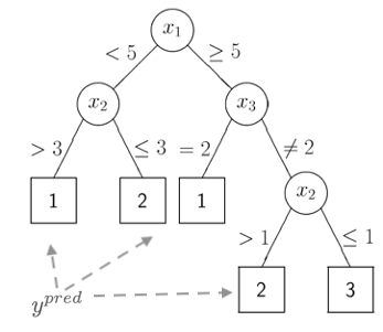
The classification and regression tree (which will be introduced later in the course) is an example of a non-parametric model. It makes no distributional assumptions on the data and increasing the amount of training data is very likely to increase the complexity of the tree.
2.5 Uncertainty
Arguably, we are living in a deterministic universe without considering quantum theory, which means the underlying system that generates the data is deterministic. One might think that the outcome of rolling dice is purely random. Actually, this is NOT true. If one can observe every related detail including for example the smoothness of the landing surface, the air resistance and the exact direction and velocity of the dice once it left the hand, one shall be able to predict the outcome precisely.
If the underlying system is deterministic, why are we studying machine learning from a probabilistic perspective, for example, we use the form \(p(\bf{y}|\bf{x})\) in supervised learning. The answer is uncertainty. There are two major sources of uncertainty.
Data uncertainty
If there are data involved, there is uncertainty induced by measurement error. You might think that well-made rulers, clocks and thermometers should be trustworthy, and give the right answers. But for every measurement - even the most careful - there is always a margin of “error”. To account for measurement error, we often use a noise model. For example \[ x=\tilde{x}+\eta\] where \(x\) is the observed value, \(\tilde{x}\) reflects the “true” value and \(\eta\) is the noise model, for example assuming \(\eta\sim N(0,1)\).
Model discrepancy
Another major source of uncertainty in modelling is due to model discrepancy. Recall the famous quote from George Box, “All models are wrong but some models are useful”. There is always a difference between the (imperfect) model used to approximate reality, and reality itself; this difference is termed model discrepancy. Therefore whatever model we construct, we usually include an error term to account for uncertainty due to model discrepancy. For example the \(\epsilon\) in the linear regression model we saw before. And we often assume \(\epsilon\) is a random draw from some distribution. \[y=b_0+b_1x+\epsilon\]
2.6 Correlation and Causation
Machine learning is not only widely used for prediction but also widely used for inference. One of the main tasks of inference is to investigate, evaluate and understand the relationship between (for example the predictor and response) variables. Let’s look at the two of the most common concepts, correlation and causation, closely related to this task.
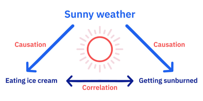
While causation and correlation can exist simultaneously, correlation does not imply causation. Causation means one thing causes another—in other words, action A causes outcome B. On the other hand, correlation is simply a relationship where action A relates to action B—but one event doesn’t necessarily cause the other event to happen.
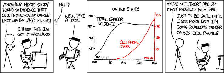
Figure 2.1: https://xkcd.com/925/
Pearson correlation coefficient
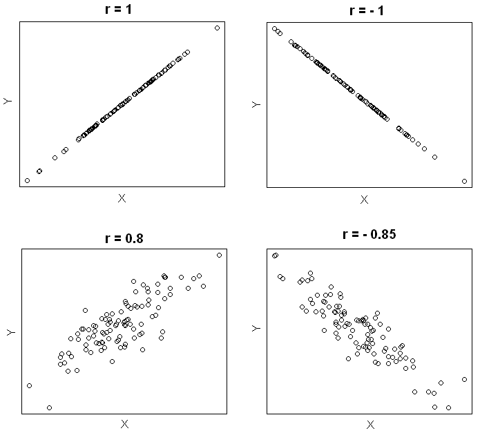
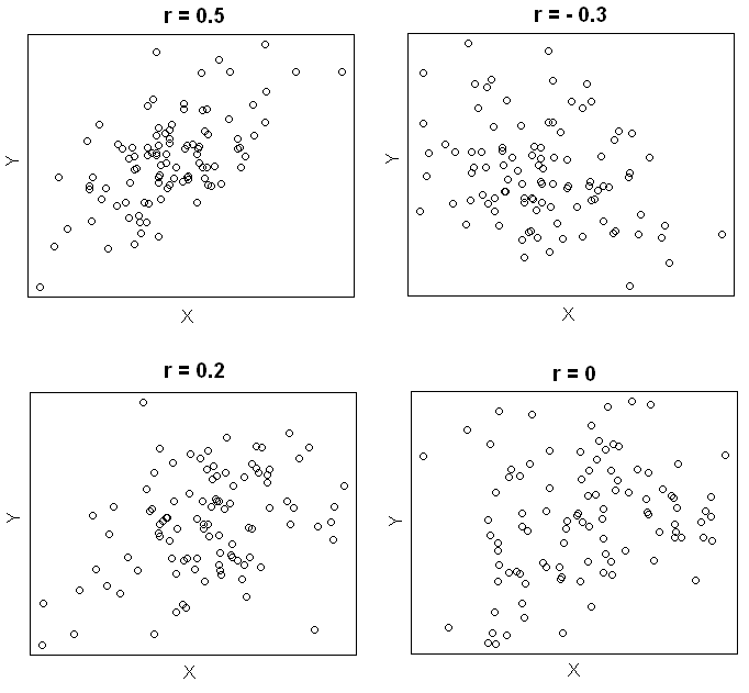
Pearson correlation coefficient(\(r\)), often called sample correlation coefficient, is a measure of the strength and the direction of a linear relationship between two variables in the sample,
\[r=\frac{\sum(x_{i} -\bar{x})(y_{i} -\bar{y}) }{\sqrt{\sum (x_{i} -\bar{x})^{2} \sum (y_{i} -\bar{y})^{2} } } \]
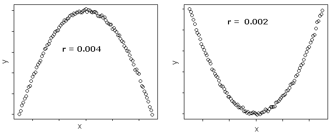
where \(r\) always lies between -1 and 1. Values of \(r\) near -1 or 1 indicate a strong linear relationship between the variables whereas values of \(r\) near 0 indicate a weak linear relationship between variables. If \(r\) is zero the variables are linearly uncorrelated, that is there is no linear relationship between the two variables.