Problem Sheets

Problem Sheet 1

Q1

Which of the following problem correspond to supervised learning? More than one correct answer can be chosen.

Given a dataset of 60,000 small square 28×28 pixel grayscale images of handwritten single digits between 0 and 9. Classify an image of a handwritten single digit into one of 10 classes representing integer values from 0 to 9.
Find clusters of genes that interact with each other
Find an investment portfolio that is likely to make a profit in the coming month
Predict whether a website user will click on an ad

Q2

Which of the following statement about parametric and non-parametric models is not true? Select all that apply:

A parametric approach reduces the problem of estimating a functional form \(f\) down to the problem of estimating a set of parameters because it assumes a form for \(f\).
A non-parametric approach does not assume a functional form \(f\) and so does not require a large number of observations to estimate \(f\).
The advantages of a parametric approach to regression or classification are the simplifying of modelling \(f\) to a few parameters and therefore the estimations of the model parameters are more accurate compared to a non-parametric approach.
The disadvantages of a parametric approach to regression or classification are a potential to inaccurately estimate \(f\) if the form of \(f\) assumed is wrong or to overfit the observations if more complex models are used.

Q3

Why is linear regression important to understand? Select all that apply:

Linear regression is very extensible and can be used to capture nonlinear effects
The linear model is often correct
The linear model is hardly ever a good representation of the underlying system, but it is an important piece in many more complex methods
Understanding simpler methods sheds light on more complex ones

Q4

Suppose that we build a simple linear regression \(Y=\beta_0+\beta_1 X+\epsilon\) based on \(n\) observations \((x_1,y_1)\),…,\((x_n,y_n)\). Which of the following indicates a fairly strong relationship between \(X\) and \(Y\)? More than one correct answer can be chosen.

The \(p\)-value for the null hypothesis \(\beta_1 = 0\) is 0.0001
The estimated parameters \(\hat{\beta}_1>>1\) and \(\hat{\beta}_0\approx 0\)
\(R^2 = 0.9\)
The \(t\)-statistic for the null hypothesis \(\beta_1 = 0\) is 40

Q5

In the case of simple linear regression, show that the least squares line always passes through the point (\(\bar{x}\),\(\bar{y}\)).

Q6

Consider a simple linear regression problem, prove that under the standard four assumptions (listed in the lecture notes), maximum likelihood estimation (MLE) is equivalent to the least squares estimation (LSE) of the model parameters.

Q7

A company manufactures an electronic device to be used in a very wide temperature range. The company knows that increased temperature shortens the lifetime of the device, and a study is therefore performed in which the lifetime is determined as a function of temperature. The following data is found:

Temperature in Celcius	Lifetime in hours
10	420
20	365
30	285
40	220
50	176
60	117
70	69
80	34
90	5

Construct a linear regression model for this problem. Estimate the model parameters. Calculate the 95% confidence interval for the slope in the linear regression model.

Q8

Consider a simple linear regression model, fit by least squares to a set of training data \((x_1,y_1),...,(x_N,y_N)\) drawn at random from a population. Let \(\hat{\beta}_0\) and \(\hat{\beta}_1\) be the least squares estimates. Suppose we have some test data \((x'_1,y'_1),...,(x'_M,y'_M)\) drawn at random from the same population as the training data. Prove that \[ E[\frac{1}{N}\sum_{i=1}^{N}(y_i-\hat{\beta}_0-\hat{\beta}_1 x_i)^2]\leq E[\frac{1}{M}\sum_{i=1}^{M}(y'_i-\hat{\beta}_0-\hat{\beta}_1 x'_i)^2] \]

Problem Sheet 1 Solution

Q1

Which of the following problem correspond to supervised learning? More than one correct answer can be chosen.

Given a dataset of 60,000 small square 28×28 pixel grayscale images of handwritten single digits between 0 and 9. Classify an image of a handwritten single digit into one of 10 classes representing integer values from 0 to 9.
Find clusters of genes that interact with each other
Find an investment portfolio that is likely to make a profit in the coming month
Predict whether a website user will click on an ad

Solution: A, C, D

Q2

Which of the following statement about parametric and non-parametric models is not true? Select all that apply:

A parametric approach reduces the problem of estimating a functional form \(f\) down to the problem of estimating a set of parameters because it assumes a form for \(f\).
A non-parametric approach does not assume a functional form \(f\) and so does not require a large number of observations to estimate \(f\).
The advantages of a parametric approach to regression or classification are the simplifying of modelling \(f\) to a few parameters and therefore the estimations of the model parameters are more accurate compared to a non-parametric approach.
The disadvantages of a parametric approach to regression or classification are a potential to inaccurately estimate \(f\) if the form of \(f\) assumed is wrong or to overfit the observations if more complex models are used.

Solution: B, C

Q3

Why is linear regression important to understand? Select all that apply:

Linear regression is very extensible and can be used to capture nonlinear effects
The linear model is often correct
The linear model is hardly ever a good representation of the underlying system, but it is an important piece in many more complex methods
Understanding simpler methods sheds light on more complex ones

Solution: A, C, D

Q4

The \(p\)-value for the null hypothesis \(\beta_1 = 0\) is 0.0001
The estimated parameters \(\hat{\beta}_1>>1\) and \(\hat{\beta}_0\approx 0\)
\(R^2 = 0.9\)
The \(t\)-statistic for the null hypothesis \(\beta_1 = 0\) is 40

Solution: C

Q5

In the case of simple linear regression, show that the least squares line always passes through the point (\(\bar{x}\),\(\bar{y}\)).

Solution: Simply using the formular of the linear square estimate of \(\beta_0\), \(\hat{\beta_0}=\bar{y}-\hat{\beta_1}\bar{x}\).

Q6

Consider a simple linear regression problem, proof that under the standard four assumptions (listed in the lecture notes), maximum likelihood estimation (MLE) is equivalent to the least squares estimation (LSE) of the model parameters.

Solution: Given the IID and normality distribution, the log-likelihood function can be written as follows: \[ l(\boldsymbol{\beta})=\sum \log p(y_i|x_i,\boldsymbol{\beta}) \] \[\begin{equation} \begin{split} l(\hat{\boldsymbol{\beta}}) & = \sum \log p(y_i|x_i,\hat{\boldsymbol{\beta}})\\ & = \sum \log\left[\left(\frac{1}{2\pi \sigma^2}\right)^{\frac{1}{2}}\exp\left(-\frac{1}{2\sigma^2}\left(y_i-(\hat{\beta}_0+\hat{\beta}_1 x_i)\right)^2\right)\right]\\ & \propto -\frac{1}{2\sigma^2} SSE(\hat{\boldsymbol{\beta}}) \end{split} \end{equation}\]

Q7

Temperature in Celcius	Lifetime in hours
10	420
20	365
30	285
40	220
50	176
60	117
70	69
80	34
90	5

Construct a linear regression model for this problem. Estimate the model parameters. Calculate the 95% confidence interval for the slope in the linear regression model.

Solution:

\(\hat{\beta}_0=453.556\) and \(\hat{\beta}_1=-5.313\)

Confidence interval: \((-5.915, -4.705)\)

Q8

Solution:

Note \[ E[\frac{1}{M}\sum_{i=1}^{M}(y'_i-\hat{\beta}_0-\hat{\beta}_1 x'_i)^2]=E[(y'_i-\hat{\beta}_0-\hat{\beta}_1 x'_i)^2] \] since for IID random variables \(z_i\), \[ E[\frac{1}{n}\sum_{i=1}^{n}z_i]=E(z) \]

Therefore, it doesn’t matter whether we have \(M\) test points or \(N\) test points, i.e. \[ E[\frac{1}{M}\sum_{i=1}^{M}(y'_i-\hat{\beta}_0-\hat{\beta}_1 x'_i)^2]=E[\frac{1}{N}\sum_{i=1}^{N}(y'_i-\hat{\beta}_0-\hat{\beta}_1 x'_i)^2] \]

Define the random variables:

\(A=\frac{1}{N}\sum_{i=1}^{N}(y_i-\hat{\beta}_0-\hat{\beta}_1 x_i)^2\) and \(B=\frac{1}{N}\sum_{i=1}^{N}(y'_i-\tilde{\beta}_0-\tilde{\beta}_1 x'_i)^2\) where \(\tilde{\beta}_0\) and \(\tilde{\beta}_1\) are the LS estimates of the linear regression parameters based on the TEST set. Note that \(\{y_i,x_i\}\) and \(\{y'_i,x'_i\}\) are samples from the same distribution, hence \(A\) and \(B\) have the same distribution and \(E(A)=E(B)\).

As \(\tilde{\beta}_0\) and \(\tilde{\beta}_1\) are the LS estimates, \[ B=\frac{1}{N}\sum_{i=1}^{N}(y'_i-\tilde{\beta}_0-\tilde{\beta}_1 x'_i)^2\leq \frac{1}{N}\sum_{i=1}^{N}(y'_i-\hat{\beta}_0-\hat{\beta}_1 x'_i)^2 \]

Therefore \[ E\left[\frac{1}{N}\sum_{i=1}^{N}(y_i-\hat{\beta}_0-\hat{\beta}_1 x_i)^2\right]=E\left[\frac{1}{N}\sum_{i=1}^{N}(y'_i-\tilde{\beta}_0-\tilde{\beta}_1 x'_i)^2\right]\leq E\left[\frac{1}{N}\sum_{i=1}^{N}(y'_i-\hat{\beta}_0-\hat{\beta}_1 x'_i)^2 \right] \]

Problem Sheet 2

Q1

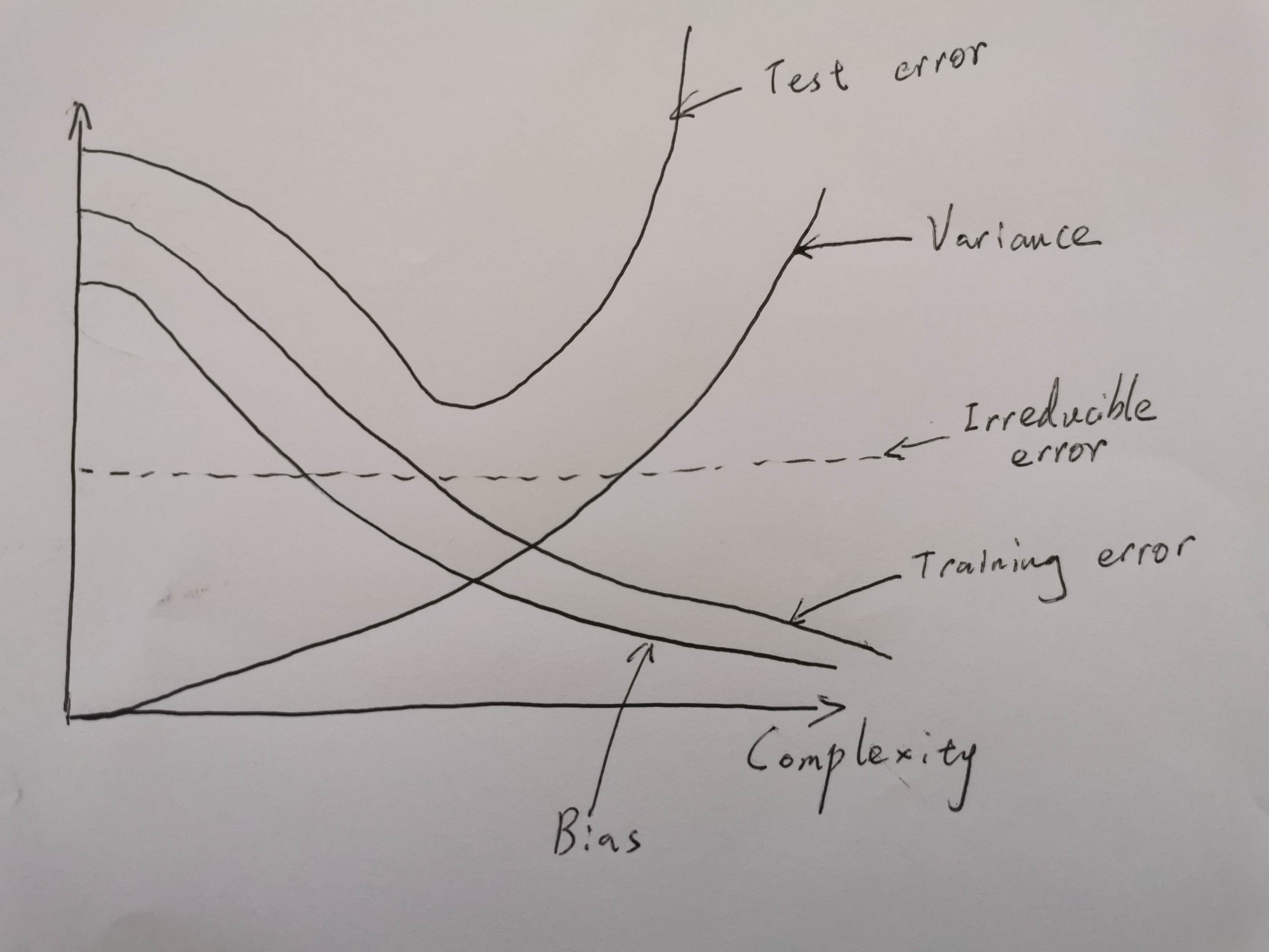
Make a sketch of typical squared bias, variance, irreducible error, training error and test error curves (i.e. five curves) on a single graph, where the x-axis represents the complexity of the model and the y-axis represents the values for each curve. Explain why each of the five curves has the shape sketched.

Q2

Which of the following statement about modelling is NOT true? Select all that apply:

A fitted model with more predictors will necessarily have a lower training error than a model with fewer predictors.
The advantage of building a very complex model for regression or classification is obtaining a better fit to the data which will lead to smaller test error.
The disadvantages for a very complex approach for regression or classification are i) requires estimating a greater number of parameters; ii) follows the noise too closely which might lead to overfitting.
A more complex model would usually be preferred to a less complex approach when we are interested in prediction and not the interpretability of the results.

Q3

You are fitting a linear regression model to a data set. The model has up to 10 predictors and 100 observations. Which of the following is NOT true in terms of using the model selection criteria to select a number of predictors to include?

Mallows’ \(C_p\) will likely select a model with more predictors than AIC
Mallows’ \(C_p\) will select the same model as AIC
Mallows’ \(C_p\) will likely select a model with fewer predictors than BIC
Mallows’ \(C_p\) will likely select a model with more predictors than BIC

Q4

Following Q3, which of the model selection approach will lead to the smallest test MSE?

Forward Stepwise Selection
Backward Stepwise Selection
Best Subset Selection
Not enough information

Q5

Following Q3, if you decide to use Best Subset Selection to decide which predictors to include, how many different models will you end up considering? How many if you use Forward Stepwise Selection?

Q6

Which of the following statement about multicollinearity is TRUE? Select all that apply:

A. When predictors are correlated, it indicates that changes in one predictor are associated with shifts in another predictor. The stronger the correlation, the more difficult it is to change one predictor without changing another.

B. When predictors are highly correlated, the coefficient estimates become very sensitive to small changes in the model.

C. Multicollinearity reduces the precision of the estimated coefficients, which weakens the statistical power of the regression model. One might not be able to trust the p-values to identify independent variables that are statistically significant.

D. Multicollinearity does not influence the predictions, precision of the predictions. If the primary goal is to make predictions without understanding the role of each predictor, there is no need to reduce multicollinearity.

Q7

Consider a simple linear regression problem, prove that under the standard four assumptions (listed in the lecture notes):

The least square estimates \(b_0\) and \(b_1\) are unbiased estimates.
The variances of the least squares estimators in simple linear regression are:

\[Var[b_0]=\sigma^2_{b_0}=\sigma^2\left(\frac{1}{n}+\frac{\bar{x}^2}{S_{xx}}\right)\]

\[Var[b_1]=\sigma^2_{b_1}=\frac{\sigma^2}{S_{xx}}\]

The covariance of the least squares estimators in simple linear regression is: \[Cov[b_0,b_1]=\sigma_{b_0,b_1}=-\sigma^2\frac{\bar{x}}{S_{xx}}\]

Q8

Suppose that you work part-time at a bowling alley that is open daily from noon to midnight. Although business is usually slow from noon to 6 P.M., the owner has noticed that it is better on hotter days during the summer, perhaps because the premises are comfortably air-conditioned. The owner shows you some data that she gathered last summer. This data set includes the maximum temperature (in Fahrenheit) and the number of lines bowled between noon and 6 P.M. for each of 20 days. (The maximum temperatures ranged from \(77^{\circ}F\) to \(95^{\circ}F\) during this period.) The owner would like to know if she can estimate tomorrow’s business from noon to 6 P.M. by looking at tomorrow’s weather forecast. She asks you to analyze the data. Let \(x\) be the maximum temperature for a day and \(y\) the number of lines bowled between noon and 6 P.M. on that day. The computer output based on the data for 20 days provided the following results: \[ \hat{y}=-432+7.7x, \;\;\; s_e=28.17,\;\;\; Sxx=607,\; and\; \bar{x}=87.5 \] Assume that the weather forecasts are reasonably accurate.

Does the maximum temperature seem to be a useful predictor of bowling activity between noon and 6 P.M.? Use an appropriate statistical procedure based on the information given. Use \(\alpha=0.05\).
The owner wants to know how many lines of bowling she can expect, on average, for days with a maximum temperature of \(90^{\circ}F\). Answer using a \(95\%\) confidence level.
The owner has seen tomorrow’s weather forecast, which predicts a high of \(90^{\circ}F\). About how many lines of bowling can she expect? Answer using a \(95\%\) confidence level.
The owner asks you how many lines of bowling she could expect if the high temperature were \(100^{\circ}F\). Give a point estimate, together with an appropriate warning to the owner.

Problem Sheet 2 Solution

Q1

Q2

Which of the following statement about modelling is NOT true? Select all that apply:

A fitted model with more predictors will necessarily have a lower training error than a model with fewer predictors.
The advantage of building a very complex model for regression or classification is obtaining a better fit to the data which will lead to smaller test error.
The disadvantages for a very complex approach for regression or classification are i) requires estimating a greater number of parameters; ii) follows the noise too closely which might lead to overfitting.
A more complex model would usually be preferred to a less complex approach when we are interested in prediction and not the interpretability of the results.

Solution: A, B For A, note the two models may be structurally different and do not share predictors at all. For B, not necessarily lead to small TEST error.

Q3

Mallows’ \(C_p\) will likely select a model with more predictors than AIC
Mallows’ \(C_p\) will select the same model as AIC
Mallows’ \(C_p\) will likely select a model with fewer predictors than BIC
Mallows’ \(C_p\) will likely select a model with more predictors than BIC

Solution: A, C

Q4

Following Q3, which of the model selection approach will lead to the smallest test MSE?

Forward Stepwise Selection
Backward Stepwise Selection
Best Subset Selection
Not enough information

Solution: D

Q5

Following Q3, if you decide to use Best Subset Selection to decide which predictors to include, how many different models will you end up considering? How many if you use Forward Stepwise Selection?

Solution: i) \(2^{10}=1024\) ii) \(1+\frac{10\times(10+1)}{2}=56\)

Q6

Which of the following statement about multicollinearity is TRUE? Select all that apply:

B. When predictors are highly correlated, the coefficient estimates become very sensitive to small changes in the model.

Solution: A, B, C, D

Q7

Consider a simple linear regression problem, prove that under the standard four assumptions (listed in the lecture notes):

The least square estimates \(b_0\) and \(b_1\) are unbiased estimates.
The variances of the least squares estimators in simple linear regression are:

\[Var[b_0]=\sigma^2_{b_0}=\sigma^2\left(\frac{1}{n}+\frac{\bar{x}^2}{S_{xx}}\right)\]

\[Var[b_1]=\sigma^2_{b_1}=\frac{\sigma^2}{S_{xx}}\]

The covariance of the least squares estimators in simple linear regression is: \[Cov[b_0,b_1]=\sigma_{b_0,b_1}=-\sigma^2\frac{\bar{x}}{S_{xx}}\]

Solution:

Note all the expectation and variance is conditioned on \(X\) is known.

Proof of \(E[b_1]=\beta_1\) see lecture notes
Proof of \(E[b_0]=\beta_0\) \[\begin{equation} \begin{split} E(b_0) & = E\left(\bar{y}-b_1\bar{x}\right)\\ & = \frac{1}{n}\sum E(y_i)-E(b_1 \bar{x}) \\ & = \frac{1}{n}\sum (\beta_0+\beta_1 x_i)-E(b_1)\frac{1}{n}\sum x_i \\ & = \frac{1}{n}\sum (\beta_0+\beta_1 x_i)-\beta_1 \frac{1}{n}\sum x_i \\ & = \beta_0 \end{split} \end{equation}\]
Proof of \(Var[b_0]\) see lecture notes
Proof of \(Var[b_1]\) see lecture notes
Proof of \(Cov[b_0,b_1]\) \[\begin{equation} \begin{split} Cov[b_0,b_1] & = Cov[\bar{y}-\bar{x}b_1,b_1]\\ & = Cov[\bar{y},b_1]-\bar{x}Cov[b_1,b_1] \\ & = 0 - \bar{x} Var(b_1) \\ & = -\bar{x}\frac{\sigma^2}{S_{xx}} \end{split} \end{equation}\] See the lecture notes of proof \(Var[b_1]\) for the proof of \(Cov[\bar{y},b_1]=0\).

Q8

Does the maximum temperature seem to be a useful predictor of bowling activity between noon and 6 P.M.? Use an appropriate statistical procedure based on the information given. Use \(\alpha=0.05\).
The owner wants to know how many lines of bowling she can expect, on average, for days with a maximum temperature of \(90^{\circ}F\). Answer using a \(95\%\) confidence level.
The owner has seen tomorrow’s weather forecast, which predicts a high of \(90^{\circ}F\). About how many lines of bowling can she expect? Answer using a \(95\%\) confidence level.
The owner asks you how many lines of bowling she could expect if the high temperature were \(100^{\circ}F\). Give a point estimate, together with an appropriate warning to the owner.

Solution:

\(\hat{y}=-432+7.7x, \;\;\; s_e=28.17,\;\;\; Sxx=607,\; and\; \bar{x}=87.5\)

\(b_1=7.7\), \(s_{b_1}=s_e/\sqrt{S_{xx}}=28.17/\sqrt{607}=1.1434\)

Test: \(H_0:\; \beta_1=0\) vs \(H_1:\; \beta_1>0\)

Use \(t\) distribution with \(df=n-2=20-2=18\)

For \(\alpha=0.05\), the critical value \(t^*=1.734\)

\(t_{stats}=(7.7-0)/1.1434=6.734>t^*\)

Reject \(H_0\), there is sufficient evidence to conclude \(\beta_1\) is positive, i.e. the maximum temperature and bowling activity between twelve noon and 6:00 pm have a positive association.
For \(x^*=90\), \(\hat{y}^*=-432+7.7(90)=261\)

\(s_{ci}=s_e\sqrt{\frac{1}{n}+\frac{(x^*-\bar{x})^2}{S_xx}}=28.17\sqrt{\frac{1}{20}+\frac{(90-87.5)^2}{607}}=6.9172\)

The \(95\%\) confidence interval for \(u^*|x^*=90\) is

\(\hat{y}^*\pm t_{\alpha/2} s_{ci}=261\pm2.101(6.9172)->(246.4670,275.5330)\)
\(s_{pi}=s_e\sqrt{1+\frac{1}{n}+\frac{(x^*-\bar{x})^2}{S_xx}}=28.17\sqrt{1+\frac{1}{20}+\frac{(90-87.5)^2}{607}}=29.0068\)

The \(95\%\) prediction interval for \(y^*\) is

\(\hat{y}^*\pm t_{\alpha/2} s_{pi}=261\pm2.101(29.0068)->(200.0567,321.9433)\)
\(y^* = –432 + 7.7(100) = 338\) lines

Our regression line is only valid for the range of x values in our sample (\(77^{\circ}F\) to \(95^{\circ}F\)). We should interpret this estimate very cautiously and not attach too much value to it.

Problem Sheet 3

Q1

Suppose we estimate the regression coefficients in a linear regression model by minimizing \[\sum_{i=1}^{n} \Bigg( y_i - \beta_0 - \sum_{j=1}^{p}\beta_j x_{ij}\Bigg)^2 + \lambda\sum_{j=1}^p\beta_j^2\] for a particular value of \(\lambda\). Which of the following statement is TRUE? Select all that apply:

A. As we increase \(\lambda\) from 0, the training RSS will steadily increase.

B. As we increase \(\lambda\) from 0, the test RSS will steadily decrease.

C. As we increase \(\lambda\) from 0, the (squared) bias will steadily decrease.

D. As we increase \(\lambda\) from 0, the variance of fitted values will steadily decrease.

Q2

Which of the following is a benefit of the sparsity imposed by the Lasso? Select all that apply:

Sparse models are generally more easy to interpret.
The Lasso does variable selection by default.
Using the Lasso penalty helps to decrease the bias of the fits.
Using the Lasso penalty helps to decrease the variance of the fits.

Q3

You perform a regression on a problem where your second predictor, x_2, is measured in meter. You decide to refit the model after changing x_2 to be measured in kilometer. Which of the following is true? Select all that apply:

If the model you performed is standard linear regression, then \(\hat{\beta}_2\) will change but \(\hat{y}\) will remain the same.
If the model you performed is standard linear regression, then neither \(\hat{\beta}_2\) nor \(\hat{y}\) will change.
If the model you performed is ridge regression, then \(\hat{\beta}_2\) and \(\hat{y}\) will both change.
If the model you performed is Lasso regression, then neither \(\hat{\beta}_2\) nor \(\hat{y}\) will change.

Q4

You are working on a regression problem with many variables, so you decide to do Principal Components Analysis first and then fit the regression to the first 2 principal components. Which of the following would you expect to happen? Select all that apply:

A subset of the features will be selected.
Model Bias will decrease relative to the full least squares model.
Variance of fitted values will decrease relative to the full least squares model.
Model interpretability will improve relative to the full least squares model.

Q5

We compute the principal components of our p predictor variables. The RSS in a simple linear regression of Y onto the largest principal component will always be no larger than the RSS in a simple regression of Y onto the second largest principal component. True or False?

Q6

Suppose we estimate the regression coefficients for a lasso regression model of a single predictor \(x\) for by minimizing \[\sum_{i=1}^{n} \Bigg( y_i - \beta_0 - \beta_1 x_{i}\Bigg)^2\] subject to \(|\beta_1|\leq c\). For a given \(c\), the fitted coefficient for predictor \(x\) is \(\hat{\beta}_1=\alpha\). Suppose we now include an exact copy \(x^*=x\) and refit our lasso regression. Characterize the effect of this exact collinearity by describing the set of solutions for \(\hat{\beta}_1\) and \(\hat{\beta}^*_1\), using the same value of \(c\).

Q7

It is well-known that ridge regression tends to give similar coefficient values to correlated variables, whereas the lasso may give quite different coefficient values to correlated variables. We will now explore this property in a very simple setting. Suppose that \(n = 2\), \(p = 2\), \(x_{11} = x_{12}\), \(x_{21} = x_{22}\). Furthermore, suppose that \(y_1 +y_2 = 0\) and \(x_{11} +x_{21} = 0\) and \(x_{12} +x_{22} = 0\), so that the estimate for the intercept in a least squares, ridge regression, or lasso model is zero: \(\hat{\beta}_0 = 0\).

Write out the ridge regression optimization problem in this setting.
Argue that in this setting, the ridge coefficient estimates satisfy \(\hat{\beta}_1 = \hat{\beta}_2\).
Write out the lasso optimization problem in this setting.
Argue that in this setting, the lasso coefficients \(\hat{\beta}_1\) and \(\hat{\beta}_2\) are not unique—in other words, there are many possible solutions to the optimization problem in (c). Describe these solutions.

Q8

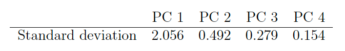
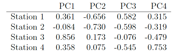
A principal component analysis of a 4-dimensional data set (containing the annual power generations of four power stations over a 20 years period) has been carried out. The standard deviation of each of the principal component (PC) is listed below: The eigenvectors generated using principal component analysis are listed below:

Let \(\hat{\boldsymbol{\Sigma}}\in\mathbb{R}^{4\times4}\) denote the sample variance matrix of the data set.

Outline the main goals of principal components analysis of data
Provide the ordered eigenvalues of \(\hat{\boldsymbol{\Sigma}}\), and given the total variance of the data cloud.
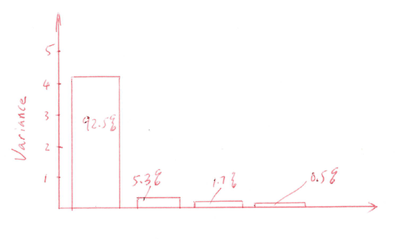
Draw a scree plot. How many components would you need in order to capture at least \(95\%\) of the total variance of the data cloud?
Provide the first and the second eigenvector of \(\hat{\boldsymbol{\Sigma}}\), which we denote by \(\boldsymbol{\gamma_1}\) and \(\boldsymbol{\gamma_2}\). Without carrying out calculations, give the numerical values of \(\boldsymbol{\gamma_1}^T\boldsymbol{\gamma_1}\), \(\boldsymbol{\gamma_2}^T\boldsymbol{\gamma_1}\) and \(\boldsymbol{\gamma_2}^T\boldsymbol{\gamma_2}\), and explain your answer.

Problem Sheet 3 Solution

Q1

A. As we increase \(\lambda\) from 0, the training RSS will steadily increase.

B. As we increase \(\lambda\) from 0, the test RSS will steadily decrease.

C. As we increase \(\lambda\) from 0, the (squared) bias will steadily decrease.

D. As we increase \(\lambda\) from 0, the variance of fitted values will steadily decrease.

Solution A, D

Q2

Which of the following is a benefit of the sparsity imposed by the Lasso? Select all that apply:

Sparse models are generally more easy to interpret.
The Lasso does variable selection by default.
Using the Lasso penalty helps to decrease the bias of the fits.
Using the Lasso penalty helps to decrease the variance of the fits.

Solution: A, B, D

Q3

If the model you performed is standard linear regression, then \(\hat{\beta}_2\) will change but \(\hat{y}\) will remain the same.
If the model you performed is standard linear regression, then neither \(\hat{\beta}_2\) nor \(\hat{y}\) will change.
If the model you performed is ridge regression, then \(\hat{\beta}_2\) and \(\hat{y}\) will both change.
If the model you performed is Lasso regression, then neither \(\hat{\beta}_2\) nor \(\hat{y}\) will change.

Solution: A, C

Q4

A subset of the features will be selected.
Model Bias will decrease relative to the full least squares model.
Variance of fitted values will decrease relative to the full least squares model.
Model interpretability will improve relative to the full least squares model.

Solution: C

Q5

Solution: False

Q6

Solution:

Apply the Lagrange multiplier, we minimize for the Lasso optimization is \[\sum_{i=1}^{n} \Bigg( y_i - \beta_0 - \beta_1 x_{i}-\beta_1^* x_i^*\Bigg)^2+\lambda( |\beta_1|+|\beta_1^*|)\] \[=\sum_{i=1}^{n} \Bigg( y_i - \beta_0 - (\beta_1+\beta_1^*) x_{i}\Bigg)^2+\lambda |\beta_1+\beta_1^*|+\lambda\left(|\beta_1|+|\beta_1^*|-|\beta_1+\beta_1^*|\right)\] Note that the first two terms represent the same minimization problem for the original lasso regression (before we added a duplicate feature) and because \[|\beta_1+\beta_1^*|\leq|\beta_1|+|\beta_1^*|,\] the third term is either positive or zero. It will be zero if \(\beta_1\) and \(\beta_1^*\) are either both positive or negative. We know that the minimum of the first two terms of this objective function happens for the solution \(\beta_1+\beta_1^*= a\) as mentioned in the problem. Therefore the solution must satisfy \(\beta_1+\beta_1^*= a\) and \(\beta_1*\beta_1^*>0\).

Q7

Write out the ridge regression optimization problem in this setting.
Argue that in this setting, the ridge coefficient estimates satisfy \(\hat{\beta}_1 = \hat{\beta}_2\).
Write out the lasso optimization problem in this setting.
Argue that in this setting, the lasso coefficients \(\hat{\beta}_1\) and \(\hat{\beta}_2\) are not unique—in other words, there are many possible solutions to the optimization problem in (c). Describe these solutions.

Solution:

\((y_1−\beta_1 x_{11}−\beta_2x_{12})^2+(y_2−\beta_1x_{21}−\beta_2x_{22})^2+\lambda(\beta_1^2+\beta_2^2)\)
Let \(x_{11} = x_{12}=x_1\), \(x_{21} = x_{22}=x_2\). Take derivatives of the expression in (a) with respect to both \(\beta_1\) and \(\beta_2\) and setting them equal to zero gives \[-2(y_1x_1+y_2x_2)+2(\hat{\beta}_1+\hat{\beta}_2)x_1^2+2(\hat{\beta}_1+\hat{\beta}_2)x_2^2+\lambda\hat{\beta}_1=0\] \[-2(y_1x_1+y_2x_2)+2(\hat{\beta}_1+\hat{\beta}_2)x_1^2+2(\hat{\beta}_1+\hat{\beta}_2)x_2^2+\lambda\hat{\beta}_2=0\] subtract one equation from the other givens \(\hat{\beta}_1=\hat{\beta}_2\)
\((y_1−\beta_1 x_{11}−\beta_2x_{12})^2+(y_2−\beta_1x_{21}−\beta_2x_{22})^2+\lambda(|\beta_1|+|\beta_2|)\)
Note that minimizing the function in (c) is equivalent to minimizing the LS subject to the constraints \(|\beta_1|+|\beta_2|\leq c\), which can be geometrically interpreted as a diamond centered at \((0,0)\).

Also given that \(y_1 +y_2 = 0\) and \(x_{11} +x_{21} = 0\) and \(x_{12} +x_{22} = 0\), the LS function \((y_1−\beta_1 x_{11}−\beta_2x_{12})^2+(y_2−\beta_1x_{21}−\beta_2x_{22})^2=2(y_1-(\beta_1+\beta_2)x_1)^2\).

Therefore the solution of minimizing LS is \(\hat{\beta}_1+\hat{\beta}_2=\frac{y_1}{x_1}\), which is in fact a line parallel to the edge of “Lasso-diamond” \(\hat{\beta}_1+\hat{\beta}_2=c\). Note the solutions to the original Lasso optimization problem are contours of the function \(2(y_1-(\hat\beta_1+\hat\beta_2)x_1)^2\) that touch the Lasso-diamond \(\hat{\beta}_1+\hat{\beta}_2=c\).

Since \(\hat{\beta}_1\) and \(\hat{\beta}_2\) are along the line \(\hat{\beta}_1+\hat{\beta}_2=\frac{y_1}{x_1}\), the entire edge \(\hat{\beta}_1+\hat{\beta}_2=c\) is a potential solution to the Lasso optimization problem! The same argument can be made for the opposite Lasso-diamond edge \(\hat{\beta}_1+\hat{\beta}_2=-c\).

Therefore this Lasso problem does not have a unique solution. The general form of solution is given by two line segments: \[\hat{\beta}_1+\hat{\beta}_2=c; \; \hat{\beta}_1\geq 0\; and \; \hat{\beta}_2\geq 0 \] \[\hat{\beta}_1+\hat{\beta}_2=-c; \; \hat{\beta}_1\leq 0\; and \; \hat{\beta}_2\leq 0 \]

Q8

Let \(\hat{\boldsymbol{\Sigma}}\in\mathbb{R}^{4\times4}\) denote the sample variance matrix of the data set.

Outline the main goals of principal components analysis of data
Provide the ordered eigenvalues of \(\hat{\boldsymbol{\Sigma}}\), and given the total variance of the data cloud.
Draw a scree plot. How many components would you need in order to capture at least \(95\%\) of the total variance of the data cloud?
Provide the first and the second eigenvector of \(\hat{\boldsymbol{\Sigma}}\), which we denote by \(\boldsymbol{\gamma_1}\) and \(\boldsymbol{\gamma_2}\). Without carrying out calculations, give the numerical values of \(\boldsymbol{\gamma_1}^T\boldsymbol{\gamma_1}\), \(\boldsymbol{\gamma_2}^T\boldsymbol{\gamma_1}\) and \(\boldsymbol{\gamma_2}^T\boldsymbol{\gamma_2}\), and explain your answer.

Solution:

To assess “true” dimensionality of multivariate data

To provide low-dimensional representations of data

To relate principal forms of variation to original variables

To provide principal components that are uncorrelated with each other.
\(\lambda_1=2.056^2=4.227136\)

\(\lambda_2=0.492^2=0.242064\)

\(\lambda_3=0.279^2=0.077841\)

\(\lambda_4=0.154^2=0.023716\)

\(TV=\lambda_1+\lambda_2+\lambda_3+\lambda_4=4.570757\)
We need the first two components to capture at least \(95\%\) of the total variance.
\(\boldsymbol{\gamma}_1=(0.361,-0.084,0.856,0.358)^T\); \(\boldsymbol{\gamma}_2=(-0.656,-0.730,0.173,0.075)^T\).

eigenvectors are unit vectors, i.e \(\boldsymbol{\gamma}_1^T\boldsymbol{\gamma}_1=\boldsymbol{\gamma}_2^T\boldsymbol{\gamma}_2=1\) and mutually orthogonal, i.e. \(\boldsymbol{\gamma}_2^T\boldsymbol{\gamma}_1=0\).

Problem Sheet 4

Q1

Which of the following statement about smoothing splines is TRUE? Select all that apply:

A. Smoothing splines are natural cubic splines with an infinite number of knots.

B. Letting tuning parameter \(\lambda\) tend to infinity leads to the standard (first-order) linear model situation.

C. Too small values of \(\lambda\) could lead to overfitting.

D. \(\lambda\) can be tuned via cross-validation.

Q2

Let \(I\{x\leq c\}\) denote a function which is \(1\) if \(x\leq c\) and \(0\) otherwise.

Which of the following is a basis for linear splines with a knot at \(c\)? Select all that apply:

\(1,\; x, \; (x-c)I\{x> c\}\)
\(1,\; x, \; (x-c)I\{x\leq c\}\)
\(1,\; x, \; I\{x\leq c\}\)
\(1,\; (x-c)I\{x> c\}, \; (x-c)I\{x\leq c\}\).

Q3

Suppose we have a random sample from \(n\) individuals. For each individual we have measurements on \(p\) predictor variables \((X_1,...,X_p)\) and a binary response variable \(Y\). A logistic regression model is fitted to the data. Choose all TRUE statements about logistic regression.

A. Logistic regression is based on a conditional model for \((X_1,...,X_p)|Y=0\) and \((X_1,...,X_p)|Y=1\)

B. If the coefficient of the j-th predictor variable, \(\beta_j\), is positive, the probability that the response variable \(Y\) is equal to \(1\) increases as \(x_j\) increases whilst all other predictor variables remain the same.

C. Logistic regression cannot use categorical variables as predictor variables.

D. Logistic regression cannot be extended to handle categorical response variables which take more than two possible outcomes.

Q4

In terms of model complexity, which is more similar to a smoothing spline with 100 knots and 5 effective degrees of freedom?

A natural cubic spline with 5 knots
A natural cubic spline with 100 knots

Q5

In the GAM \(y\sim f_1(X_1)+f_2(X_2)+\epsilon\), as we make \(f_1\) and \(f_2\) more and more complex we can approximate any regression function to arbitrary precision. True or False?

Q6

Is the following function a cubic spline? Why or why not?

\[ f(x) = \begin{cases} 0, \qquad \qquad \qquad \qquad \qquad x<0,\\ x^3, \qquad \qquad \qquad \qquad \; \; \; \; \; 0\leq x<1, \\ x^3+(x-1)^3, \qquad \qquad \; \; 1\leq x<2, \\ -(x-3)^3-(x-4)^3, \; \; \; \; \; 2\leq x<3, \\ -(x-4)^3, \qquad \qquad \qquad 3\leq x<4, \\ 0, \qquad \qquad \qquad \qquad \; \; \; \; \;\; 4\leq x. \\ \end{cases} \]

Q7

A cubic regression spline with one knot at \(\xi\) can be obtained using a basis of the form \(x\), \(x^2\), \(x^3\), \((x - \xi)^3_+\), where \((x - \xi)^3_+=(x - \xi)^3\) if \(x>\xi\) and equals \(0\) otherwise. Show that a function of the form \[f(x)=\beta_0+\beta_1 x+ \beta_2 x^2+\beta_3 x^3+\beta_4(x - \xi)^3_+ \] is indeed a cubic regression spline, regardless of the values of \(\beta_0\), \(\beta_1\), \(\beta_2\), \(\beta_3\), \(\beta_4\).

Find a cubic polynomial \[f_1(x)=a_1+b_1x+c_1 x^2+d_1 x^3\] such that \(f(x)=f_1(x)\) for all \(x\leq\xi\). Express \(a_1,b_1,c_1,d_1\) in terms of \(\beta_0,\beta_1, \beta_2, \beta_3, \beta_4\).
Find a cubic polynomial \[f_2(x)=a_2+b_2x+c_2 x^2+d_2 x^3\] such that \(f(x)=f_2(x)\) for all \(x>\xi\). Express \(a_2,b_2,c_2,d_2\) in terms of \(\beta_0,\beta_1, \beta_2, \beta_3, \beta_4\).
Show that \(f_1(\xi)=f_2(\xi)\).
Show that \(f_1'(\xi)=f_2'(\xi)\).
Show that \(f_1''(\xi)=f_2''(\xi)\).

Q8

Prove that \(p(X)=\frac{\exp(\beta_0+\beta_1X)}{1+\exp(\beta_0+\beta_1X)}\) is equivalent to \(\ln\frac{p(X)}{1−p(X)}=\beta_0+\beta_1X\). In other words, the logistic function representation and logit transformation are equivalent.

Q9

Consider a simple logistic regression model for a binary classification problem, \(p(X)=P(Y=1|X)=\frac{\exp(\beta_0+\beta_1X)}{1+\exp(\beta_0+\beta_1X)}\). Given the data of response \(\{y_i\},i=1,...,n\) and the corresponding data of single predictor \(\{x_i\},i=1,...,n\), derive the log-likelihood of the parameters \(\beta_0,\beta_1\) and state any assumptions required for the derivation.

Problem Sheet 4 Solution

Q1

Which of the following statement about smoothing splines is TRUE? Select all that apply:

A. Smoothing splines are natural cubic splines with an infinite number of knots.

B. Letting tuning parameter \(\lambda\) tend to infinity leads to the standard (first-order) linear model situation.

C. Too small values of \(\lambda\) could lead to overfitting.

D. \(\lambda\) can be tuned via cross-validation.

Solution: B, C, D

Q2

Let \(I\{x\leq c\}\) denote a function which is \(1\) if \(x\leq c\) and \(0\) otherwise.

Which of the following is a basis for linear splines with a knot at \(c\)? Select all that apply:

\(1,\; x, \; (x-c)I\{x> c\}\)
\(1,\; x, \; (x-c)I\{x\leq c\}\)
\(1,\; x, \; I\{x\leq c\}\)
\(1,\; (x-c)I\{x> c\}, \; (x-c)I\{x\leq c\}\).

Solution: A, B, D

Q3

A. Logistic regression is based on a conditional model for \((X_1,...,X_p)|Y=0\) and \((X_1,...,X_p)|Y=1\)

C. Logistic regression cannot use categorical variables as predictor variables.

D. Logistic regression cannot be extended to handle categorical response variables which take more than two possible outcomes.

Solution: B

Q4

In terms of model complexity, which is more similar to a smoothing spline with 100 knots and 5 effective degrees of freedom?

A natural cubic spline with 5 knots
A natural cubic spline with 100 knots

Solution: A

Even though the smoothing spline has 100 knots, it is penalized to be smooth, so it is about as complex as a model with 5 variables (effective degree of freedom). The natural cubic spline with 5 knots has 5 degrees of freedom is such a model. Note a cubic spline with 5 knots has 5+3+1 degrees of freedom, the natural cubic spline adds two more linear constraints which frees 2 df at each side (a cubic polynomial model–>linear model)

Q5

In the GAM \(y\sim f_1(X_1)+f_2(X_2)+\epsilon\), as we make \(f_1\) and \(f_2\) more and more complex we can approximate any regression function to arbitrary precision. True or False?

Solution: False

Note, this additive model can not capture interaction behaviors.

Q6

Is the following function a cubic spline? Why or why not?

Solution: At \(x=2\), \(f'\) is discontinuous (15 on one side and -15 on the other side), so this is not a cubic spline.

Q7

Find a cubic polynomial \[f_1(x)=a_1+b_1x+c_1 x^2+d_1 x^3\] such that \(f(x)=f_1(x)\) for all \(x\leq\xi\). Express \(a_1,b_1,c_1,d_1\) in terms of \(\beta_0,\beta_1, \beta_2, \beta_3, \beta_4\).
Find a cubic polynomial \[f_2(x)=a_2+b_2x+c_2 x^2+d_2 x^3\] such that \(f(x)=f_2(x)\) for all \(x>\xi\). Express \(a_2,b_2,c_2,d_2\) in terms of \(\beta_0,\beta_1, \beta_2, \beta_3, \beta_4\).
Show that \(f_1(\xi)=f_2(\xi)\).
Show that \(f_1'(\xi)=f_2'(\xi)\).
Show that \(f_1''(\xi)=f_2''(\xi)\).

Solution:

For \(x\leq\xi\), \(f_1(x)\) has coefficients \(a_1=\beta_0\), \(b_1=\beta_1\), \(c_1=\beta_2\) and \(d_1=\beta_3\)
For \(x>\xi\), we have \[f(x)=β_0+β_1x+β_2x^2+β_3x^3+β_4(x−ξ)^3\] \[=(β_0−β_4ξ^3)+(β_1+3ξ^2β_4)x+(β_2−3β_4ξ)x^2+(β_3+β_4)x^3\] so we take \(a_2=β_0−β_4ξ^3\), \(b_2=β_1+3ξ^2β_4\),\(c_2=β_2−3β_4ξ\), \(d_2=\beta_3+\beta_4\).
\[f_1(ξ)=β_0+β_1ξ+β_2ξ^2+β_3ξ^3\] and \[f_2(ξ)=(β_0−β_4ξ^3)+(β_1+3ξ^2β_4)ξ+(β_2−3β_4ξ)ξ^2+(β_3+β_4)ξ^3=β_0+β_1ξ+β_2ξ^2+β_3ξ^3\]
\[f_1'(ξ)=β_1+2β_2ξ+3β_3ξ^2\] and \[f′_2(ξ)=β_1+3ξ^2β_4+2(β_2−3β_4ξ)ξ+3(β_3+β_4)ξ^2=β_1+2β_2ξ+3β_3ξ2\]
\[f″_1(ξ)=2β_2+6β_3ξ\] and \[f″_2(ξ)=2(β_2−3β_4ξ)+6(β_3+β_4)ξ=2β_2+6β_3ξ\]

Q8

Solution:

\[\begin{equation} \begin{split} \frac{p(X)}{1−p(X)} & = \frac{\frac{\exp(\beta_0+\beta_1X)}{1+\exp(\beta_0+\beta_1X)}}{1-\frac{\exp(\beta_0+\beta_1X)}{1+\exp(\beta_0+\beta_1X)}}\\ & = \frac{\frac{\exp(\beta_0+\beta_1X)}{1+\exp(\beta_0+\beta_1X)}}{\frac{1+\exp(\beta_0+\beta_1X)}{1+\exp(\beta_0+\beta_1X)}-\frac{\exp(\beta_0+\beta_1X)}{1+\exp(\beta_0+\beta_1X)}} \\ & = \frac{\frac{\exp(\beta_0+\beta_1X)}{1+\exp(\beta_0+\beta_1X)}}{\frac{1}{1+\exp(\beta_0+\beta_1X)}} \\ & = \exp(\beta_0+\beta_1X) \end{split} \end{equation}\] therefore \(\ln\frac{p(X)}{1−p(X)}=\beta_0+\beta_1X\)

Q9

Solution: The probability of the observed class was either \(p\), if \(y_i=1\), or \(1-p\), if \(y_i=0\). The likelihood is then \[L(\beta_0,\beta_1)=\prod_{i=1}^{n}p(x_i)^{y_i}(1-p(x_i))^{1-y_i}.\] The log-likelihood turns products into sums: \[\begin{equation} \begin{split} l(\beta_0,\beta_1) & = \sum_{i=1}^{n}y_i\log p(x_i)+(1-y_i)\log (1-p(x_i))\\ & =\sum_{i=1}^{n} \log (1-p(x_i))+ \sum_{i=1}^{n}y_i \log \frac{p(x_i)}{1-p(x_i)} \\ & = \sum_{i=1}^{n} \log (1-p(x_i))+ \sum_{i=1}^{n}y_i (\beta_0+\beta_1 x_i) \\ & = \sum_{i=1}^{n} -\log (1+\exp(\beta_0+\beta_1 x_i))+ \sum_{i=1}^{n}y_i (\beta_0+\beta_1 x_i) \end{split} \end{equation}\]

Note the assumptions required are

independence of observations, in order to use the \(\prod\)
\(p(X)=P(Y=1|X)=\frac{\exp(\beta_0+\beta_1X)}{1+\exp(\beta_0+\beta_1X)}\) suggests that we assume a linear relationship between the predictor \(X\) and the logit transformation of the response variable \(Y\).