Chapter 4 Model Assessment and Selection
Assessment of model performance is extremely important in practice, since it guides the choice of machine learning algorithm or model, and gives us a measure of the quality of the ultimately chosen model.
It is important to note that there are in fact two separate goals here:
Model selection: estimating the performance of different models in order to choose the best one.
Model assessment: having chosen a final model, estimating its prediction error (generalization error) over an independent new data sample.
4.1 In-sample vs out-of-sample
If we are in a data-rich situation, the best approach for both problems is to randomly divide the dataset into three parts: a training set, a validation/evaluation set, and a test set.
- The training set is used to fit the model parameters.
- The validation set is used to estimate prediction error for model selection (including choosing the values of hyperparameters).
- The test set is used for assessment of the generalization error (also referred to as test error, is the prediction error over an independent test sample.) of the final chosen model.
The period that the training set and the validation set are used for the initial parameter estimation and model selection, is called in-sample period. And an out-of-sample period uses test set to evaluate final forecasting performance.
Ideally, the test set should be kept in a “vault” and be brought out only at the end of the data analysis. Suppose instead that we use the test-set repeatedly, choosing the model with smallest test-set error. Then the test set error of the final chosen model will underestimate the true test error, sometimes substantially.
It is difficult to give a general rule on how to choose the number of observations in each of the three parts. A typical split might be \(50\%\) for training, and \(25\%\) each for validation and testing.

4.2 Cross-Validation
For the situations where there is insufficient data to split it into three parts. One could conduct k-fold Cross-validation on a single training set for both training and validation.
k-fold Cross-validation (CV) involves randomly dividing the set of \(n\) observations into \(k\) groups (or folds) of approximately equal size.
Then, for each group \(i=1,...,k\):
- Fold \(i\) is treated as a validation set, and the model is fit on the remaining \(k-1\) folds.
- The performance metric, \(Performance_i\) (for example MSE), is then computed based on the observations of the held out fold \(i\).
This process results in \(k\) estimates of the test performance, \(Performance_1,...,Performance_k\). The \(k\)-fold CV estimate is computed by averaging these values. \[CV_{(k)} = \frac{1}{k} \sum_{i=1}^{k} Performance_i \]
Figure 4.1 illustrates this nicely.
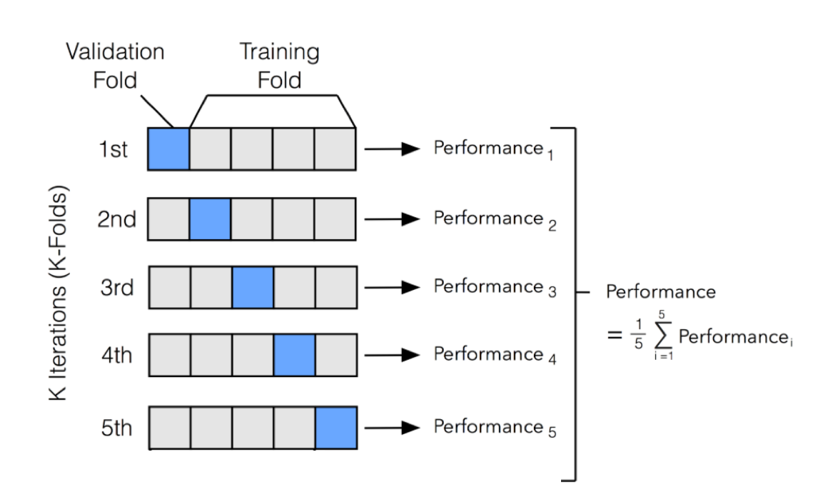
Figure 4.1: An illustration of k-fold CV with 5 folds.
The \(CV_{(k)}\) as an estimate of the test performance can also be used for model selection. Note that to assess the performance of the final chosen model, one still need another independent test sample.
4.3 Overfitting vs Underfitting
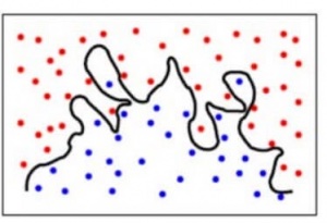
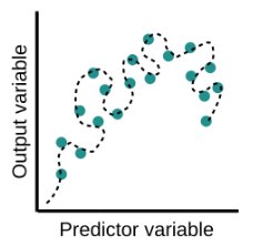
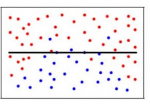
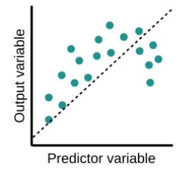
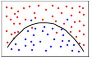
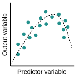
Overfitting is a common pitfall in machine learning modelling, in which a model tries to fit the training data entirely and ends up “memorizing” the data patterns and the noise/random fluctuations. These models fail to generalize and perform well in the case of unseen data scenarios, defeating the model’s purpose. That is why an overfit model results in poor test accuracy. Example of overfitting situation in classification and regression:
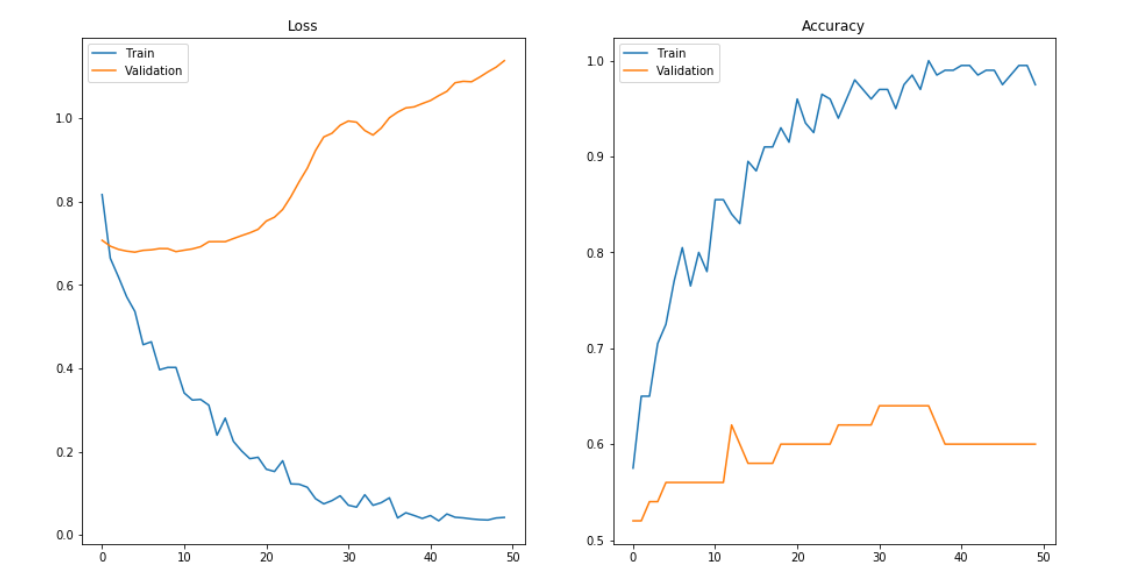
 Detecting overfitting is only possible once we move out of the training phase, for example evaluate the model performance using the validation set.
Underfitting is another common pitfall in machine learning modelling, where the model cannot create a mapping between the input and the target variable that reflects the underlying system, for example due to under-observing the features. Underfitting often leads to a higher error in the training and unseen data samples.
Example of overfitting situation in classification and regression:
Underfitting becomes obvious when the model is too simple and cannot represent a relationship between the input and the output. It is detected when the training error is very high and the model is unable to learn from the training data.
4.4 Bias Variance Trade-off
In supervised learning, the model performance can help us to identify or even quantify overfitting/underfitting. Often we use the difference between the actual values and predicted values to evaluate the model, such prediction error can in fact be decomposed into three parts:
- Bias: The difference between the average prediction of our model and the correct value which we are trying to predict. Model with high bias pays very little attention to the training data and oversimplifies the model. It always leads to high error on training and test data.
- Variance: Variance is the variability of model prediction for a given data point or a value which tells us how uncertainty our model is. Model with high variance pays a lot of attention to training data and does not generalize on the data which it hasn’t seen before. As a result, such models perform very well on training data but has high error rates on test data.
- Noise: Irreducible error that we cannot eliminate.
Mathematically, assume the relationship between the response \(Y\) and the predictors \(\boldsymbol{X}=(X_1,...,X_p)\) can be represented as:
\[ Y=f(\boldsymbol{X})+\epsilon \] where \(f\) is some fixed but unknown function of \(\boldsymbol{X}\) and \(\epsilon\) is a random error term, which is independent of \(\boldsymbol{X}\) and has mean zero.
Consider building a model \(\hat{f}(\boldsymbol{X})\) of \(f(\boldsymbol{X})\) (for example a linear regression model), the expected squared error (MSE) at a point x is
\[\begin{equation} \begin{split} MSE & = E\left[\left(y-\hat{f}(x)\right)^2\right]\\ & = E\left[\left(f(x)+\epsilon-\hat{f}(x)\right)^2\right] \\ & = E\left[\left(f(x)+\epsilon-\hat{f}(x)+E[\hat{f}(x)]-E[\hat{f}(x)]\right)^2\right] \\ & = ... \\ & = \left(f(x)-E[\hat{f}(x)]\right)^2+E\left[\epsilon^2\right]+E\left[\left(E[\hat{f}(x)]-\hat{f}(x)\right)^2\right] \\ & = \left(f(x)-E[\hat{f}(x)]\right)^2+Var[\epsilon]+Var\left[\hat{f}(x)\right]\\ & = Bias[\hat{f}(x)]^2+Var[\epsilon]+Var\left[\hat{f}(x)\right]\\ & = Bias^2+Variance+Irreducible\; Error \end{split} \end{equation}\]
We can create a graphical visualization of bias and variance using a bulls-eye diagram. Imagine that the center of the target is a model that perfectly predicts the correct values. As we move away from the bulls-eye, our predictions get worse and worse.
We can plot four different cases representing combinations of both high and low bias and variance.
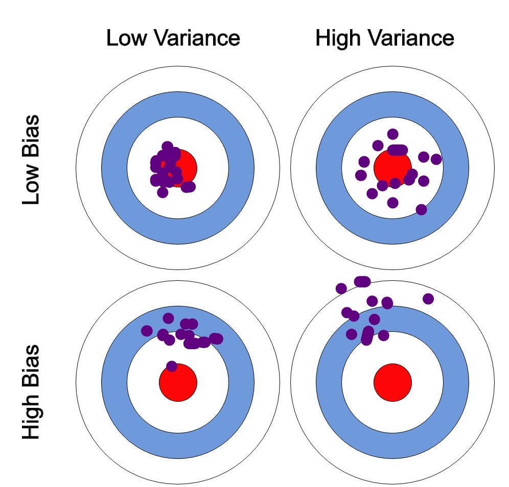
At its root, dealing with bias and variance is really about dealing with overfitting and underfitting. High bias and low variance are the most common indicators of underfitting. Similarly low bias and high variance are the most common indicators of overfitting. Bias is reduced and variance is increased in relation to model complexity. As more and more parameters are added to a model, the complexity of the model rises and variance becomes our primary concern while bias steadily falls.
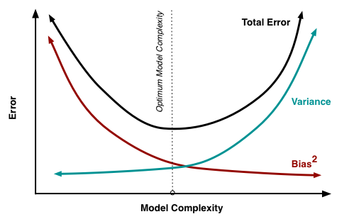
An optimal balance of bias and variance would neither overfit nor underfit the model.
Example of an optimal balanced situation in classification and regression:
4.5 Model selection for Linear regression
Consider the standard linear regression model: \[ y = \beta_0 + \beta_1x_1 + \beta_2x_2 + \ldots + \beta_p x_p +\epsilon \] Here, \(y\) is the response variable, the \(x\)’s are the predictor variables and \(\epsilon\) is an error term.
Model selection involves identifying a subset of the \(p\) predictors \(x_1,...,x_p\) of size \(d\) that we believe to be related to the response. We then fit a least squares linear regression model using just the reduced set of variables.
For example, if we believe that only \(x_1\) and \(x_2\) are related to the response, then we may take \(d=2\) and fit a model of the following form: \[ y = \beta_0 + \beta_1x_1 + \beta_2x_2 +\epsilon \] where we have deemed variables \(x_3,...,x_p\) to be irrelevant.
But how do we determine which variables are relevant? We may just `know’ which variables are most informative for a particular response (for example, from previous data investigations or talking to an expert in the field), but often we need to investigate.
How many possible linear models are we trying to choose from? Well, we will always include the intercept term \(\beta_0\). Then each variable \(X_1,...,X_p\) can either be included or not, hence we have \(2^p\) possible models to choose from.
Question: how do we choose which variables should be included in our model?
Training Error
The training error of a linear model is evaluated via the Residual Sum of Squares (RSS), which as we have seen is given by \[RSS = \sum_{i=1}^{n}(y_i - \hat{y}_i)^2,\] where \[\hat{y}_i = \hat{\beta}_0+\hat{\beta}_1x_{i1} + \hat{\beta}_2x_{i2}+ \ldots + \hat{\beta}_dx_{id}.\] is the predicted response value at input \(x_i = (x_{i1},...,x_{id})\). Or simply scaling down the RSS leads to the Mean Squared Error (MSE): \[MSE = \frac{RSS}{n}\] where \(n\) is the size of the training sample. Unfortunately, neither of these metrics is appropriate when comparing models of different dimensionality (different number of predictors) because both \(RSS\) and \(MSE\) generally decrease as we include additional predictors to a linear model. In fact, in the extreme case of \(n=p\) both metrics will be 0! This does not mean that we have a “good” model, just that we have overfitted our linear model to perfectly adjust to the training data. Overfitted models will exhibit poor predictive performance (low training error but high prediction error). Our aim is to have simple, interpretable models with relatively small \(p\) (in relation to \(n\)), which have good predictive performance.
Validation
We could simply using an independent validation set (either by splitting the data into training and validation set or using cross-validation techniques) to evaluate the model performance and select the “best” model.
For example:
Let us assume a hypothetical scenario where the true model is \[y= \beta_0 +\beta_1 x_1 +\beta_2 x_2 +\epsilon\] where \(\beta_0 = 1\), \(\beta_1 = 1.5\), \(\beta_2 = -0.5\) for some given values of the predictors \(x_1\) and \(x_2\). Let’s set the errors to be normally distributed with zero mean and variance equal to one; i.e., \(\epsilon \sim N(0,1)\). Also assume that we have three additional predictors \(x_3\), \(x_4\) and \(x_5\) which are irrelevant to \(y\) (in the sense that \(\beta_3=\beta_4=\beta_5=0\)), but of course we do not know that beforehand.
We can plot the training MSE and prediction MSE against the number of predictors used in the model, such as is illustrated in Figure 4.2.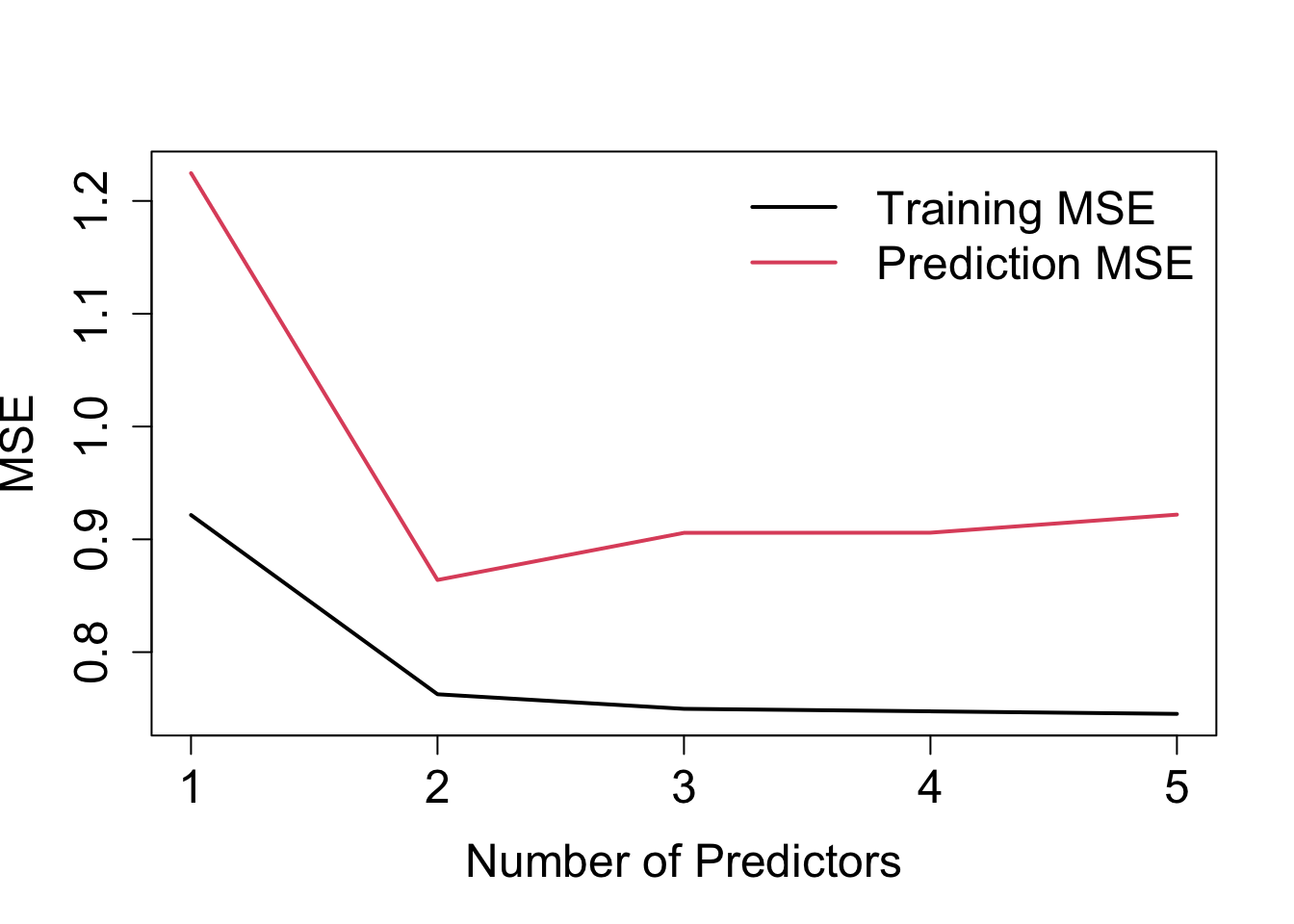
Figure 4.2: Training MSE and prediction MSE against number of predictors.
Notice the following:
- Training error: steady (negligible) decline after adding \(x_3\) – not really obvious how many predictors to include.
- Prediction error: increase after adding \(x_3\), which indicates overfitting. Clearly here one would select the model with \(x_1\) and \(x_2\)!
- Prediction errors are larger than training errors – this is generally always the case! (see Q8 in Problem Sheet 1).
4.6 Model Selection Criteria
Given that in practice we may not wish to exclude part of the data for calculating a prediction error using validation, instead of using cross-validation techniques we can also indirectly estimate prediction error by making an adjustment to the performance measure that accounts for overfitting. Here, we have several model selection criteria that are developed from such kind of adjustment.
\(C_p\)
For a given model with \(d\) predictors (out of the available \(p\) predictors) Mallows’ \(C_p\) criterion is \[C_p = \frac{1}{n}(RSS + 2 d \hat{\sigma}^2),\] where \(RSS\) is the residual sum of squares for the model of interest (with \(d\) predictors), and \(\hat{\sigma}^2=RSS_p/(n-p-1)\) is an estimate of the error variance for the full model with all \(p\) possible predictors included. As such, we use \(RSS_p\) to denote the Residual Sum of Squares for the full model with all \(p\) possible predictors included.
In practice, we choose the model which has the minimum \(C_p\) value: so we essentially penalise models of higher dimensionality (the larger \(d\) is the greater the penalty).
AIC
For linear models (with normal errors, as is often assumed), Mallows’ \(Cp\) is equivalent to the Akaike Information Criterion (AIC) (as the two are proportional), this being given by \[AIC = \frac{1}{n\hat{\sigma}^2}(RSS + 2 d \hat{\sigma}^2).\]
BIC
Another metric is the Bayesian information criterion (BIC) \[BIC = \frac{1}{n\hat{\sigma}^2}(RSS + \log(n)d \hat{\sigma}^2),\] where again the model with the minimum BIC value is selected
In comparison to \(C_p\) or AIC, where the penalty is \(2d \hat{\sigma}^2\), the BIC penalty is \(\log(n)d \hat{\sigma}^2\). This means that generally BIC has a heavier penalty (because \(\log(n)>2\) for \(n>7\)), thus BIC selects models with fewer variables than \(C_p\) or AIC.
In general, all three criteria are based on rigorous theoretical asymptotic (\(n\rightarrow \infty\)) justifications.
Adjusted R-squared value
Another simple method which is not backed up by statistical theory, but that often works well in practice, is to simply adjust the \(R^2\) metric by taking into account the number of predictors as we defined before.
The adjusted \(R^2\) value for a model with \(d\) variables is calculated as follows
\[
\mbox{Adjusted~} R^2 = 1 - \frac{RSS/(n-d-1)}{TSS/(n-1)}.
\]
In this case we choose the model with the maximum adjusted \(R^2\) value.
Example
By plotting the various model selection criteria against the number of predictors (Figure 4.3), we can see that, in our example, \(C_p\), AIC and BIC are in agreement (2 predictors). Adjusted \(R^2\) would select 3 predictors.
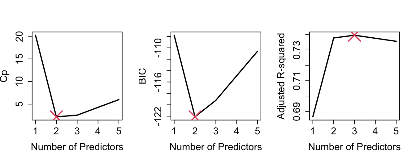
Figure 4.3: Various model selection criteria against number of predictors.
Further points
- A shortcoming of the previous approaches is that they are not applicable for models that have more variables than the size of the sample (\(d>n\)).
- Also, in the setting of penalised regression (which we will see later on in the course) deciding what \(d\) actually becomes a bit problematic.
- CV is an effective computational tool which can be used in all settings.