Practical Class Sheets 2
In this practical class, we will use R to fit linear regression models, make inference of model parameters, construct confidence intervals, assess the quality of the model, use residual diagnostic plots to assess the validity of the regression assumptions and conduct model selection for multiple linear regression.
To start, create a new R script by clicking on the corresponding menu button (in the top left); and save it somewhere in your computer. You can now write all your code into this file, and then execute it in R using the menu button Run or by simple pressing ctrl \(+\) enter.
Body Fat and Body Measurements Data
In this practical class we will investigate the dataset fat from the library faraway, which consists of 252 observations concerning percentage of body fat and body measurements. We are interested in predicting body fat (variable brozek) using the other variables available, except for siri (another way of computing body fat), density (it is used in the brozek and siri formula) and free (it is computed using the brozek formula).
\(~\)
First, we need to install the faraway package, using the command install.packages("faraway"). We only need to do this once.
Now, load the package and the data set and read the help file for more information about the variables:
library("faraway")Exploratory data analysis
To get more information about the data set:
names(fat)## [1] "brozek" "siri" "density" "age" "weight" "height" "adipos"
## [8] "free" "neck" "chest" "abdom" "hip" "thigh" "knee"
## [15] "ankle" "biceps" "forearm" "wrist"?fat
str(fat)## 'data.frame': 252 obs. of 18 variables:
## $ brozek : num 12.6 6.9 24.6 10.9 27.8 20.6 19 12.8 5.1 12 ...
## $ siri : num 12.3 6.1 25.3 10.4 28.7 20.9 19.2 12.4 4.1 11.7 ...
## $ density: num 1.07 1.09 1.04 1.08 1.03 ...
## $ age : int 23 22 22 26 24 24 26 25 25 23 ...
## $ weight : num 154 173 154 185 184 ...
## $ height : num 67.8 72.2 66.2 72.2 71.2 ...
## $ adipos : num 23.7 23.4 24.7 24.9 25.6 26.5 26.2 23.6 24.6 25.8 ...
## $ free : num 135 161 116 165 133 ...
## $ neck : num 36.2 38.5 34 37.4 34.4 39 36.4 37.8 38.1 42.1 ...
## $ chest : num 93.1 93.6 95.8 101.8 97.3 ...
## $ abdom : num 85.2 83 87.9 86.4 100 94.4 90.7 88.5 82.5 88.6 ...
## $ hip : num 94.5 98.7 99.2 101.2 101.9 ...
## $ thigh : num 59 58.7 59.6 60.1 63.2 66 58.4 60 62.9 63.1 ...
## $ knee : num 37.3 37.3 38.9 37.3 42.2 42 38.3 39.4 38.3 41.7 ...
## $ ankle : num 21.9 23.4 24 22.8 24 25.6 22.9 23.2 23.8 25 ...
## $ biceps : num 32 30.5 28.8 32.4 32.2 35.7 31.9 30.5 35.9 35.6 ...
## $ forearm: num 27.4 28.9 25.2 29.4 27.7 30.6 27.8 29 31.1 30 ...
## $ wrist : num 17.1 18.2 16.6 18.2 17.7 18.8 17.7 18.8 18.2 19.2 ...# Look at the first few rows
head(fat)## brozek siri density age weight height adipos free neck chest abdom hip
## 1 12.6 12.3 1.0708 23 154.25 67.75 23.7 134.9 36.2 93.1 85.2 94.5
## 2 6.9 6.1 1.0853 22 173.25 72.25 23.4 161.3 38.5 93.6 83.0 98.7
## 3 24.6 25.3 1.0414 22 154.00 66.25 24.7 116.0 34.0 95.8 87.9 99.2
## 4 10.9 10.4 1.0751 26 184.75 72.25 24.9 164.7 37.4 101.8 86.4 101.2
## 5 27.8 28.7 1.0340 24 184.25 71.25 25.6 133.1 34.4 97.3 100.0 101.9
## 6 20.6 20.9 1.0502 24 210.25 74.75 26.5 167.0 39.0 104.5 94.4 107.8
## thigh knee ankle biceps forearm wrist
## 1 59.0 37.3 21.9 32.0 27.4 17.1
## 2 58.7 37.3 23.4 30.5 28.9 18.2
## 3 59.6 38.9 24.0 28.8 25.2 16.6
## 4 60.1 37.3 22.8 32.4 29.4 18.2
## 5 63.2 42.2 24.0 32.2 27.7 17.7
## 6 66.0 42.0 25.6 35.7 30.6 18.8# Summary statistics
summary(fat)## brozek siri density age
## Min. : 0.00 Min. : 0.00 Min. :0.995 Min. :22.00
## 1st Qu.:12.80 1st Qu.:12.47 1st Qu.:1.041 1st Qu.:35.75
## Median :19.00 Median :19.20 Median :1.055 Median :43.00
## Mean :18.94 Mean :19.15 Mean :1.056 Mean :44.88
## 3rd Qu.:24.60 3rd Qu.:25.30 3rd Qu.:1.070 3rd Qu.:54.00
## Max. :45.10 Max. :47.50 Max. :1.109 Max. :81.00
## weight height adipos free
## Min. :118.5 Min. :29.50 Min. :18.10 Min. :105.9
## 1st Qu.:159.0 1st Qu.:68.25 1st Qu.:23.10 1st Qu.:131.3
## Median :176.5 Median :70.00 Median :25.05 Median :141.6
## Mean :178.9 Mean :70.15 Mean :25.44 Mean :143.7
## 3rd Qu.:197.0 3rd Qu.:72.25 3rd Qu.:27.32 3rd Qu.:153.9
## Max. :363.1 Max. :77.75 Max. :48.90 Max. :240.5
## neck chest abdom hip
## Min. :31.10 Min. : 79.30 Min. : 69.40 Min. : 85.0
## 1st Qu.:36.40 1st Qu.: 94.35 1st Qu.: 84.58 1st Qu.: 95.5
## Median :38.00 Median : 99.65 Median : 90.95 Median : 99.3
## Mean :37.99 Mean :100.82 Mean : 92.56 Mean : 99.9
## 3rd Qu.:39.42 3rd Qu.:105.38 3rd Qu.: 99.33 3rd Qu.:103.5
## Max. :51.20 Max. :136.20 Max. :148.10 Max. :147.7
## thigh knee ankle biceps forearm
## Min. :47.20 Min. :33.00 Min. :19.1 Min. :24.80 Min. :21.00
## 1st Qu.:56.00 1st Qu.:36.98 1st Qu.:22.0 1st Qu.:30.20 1st Qu.:27.30
## Median :59.00 Median :38.50 Median :22.8 Median :32.05 Median :28.70
## Mean :59.41 Mean :38.59 Mean :23.1 Mean :32.27 Mean :28.66
## 3rd Qu.:62.35 3rd Qu.:39.92 3rd Qu.:24.0 3rd Qu.:34.33 3rd Qu.:30.00
## Max. :87.30 Max. :49.10 Max. :33.9 Max. :45.00 Max. :34.90
## wrist
## Min. :15.80
## 1st Qu.:17.60
## Median :18.30
## Mean :18.23
## 3rd Qu.:18.80
## Max. :21.40# Check for missing values
sum(is.na(fat))## [1] 0# zero here, so no missing valuesCreate a new dataframe called fat1 which is equivalent to fat, but with the variables siri, density and free removed.
# Remove variables 2, 3 and 8.
fat1 <- fat[,-c(2,3,8)]
# siri is variable 2, density variable 3 and free variable 8.
\(~\)
Exercise 2.1
- How many rows are in this data set? How many columns? What do the rows and columns represent?
- Make some pairwise scatterplots of the predictors (columns) in this data set. Describe your findings.
- Are any of the predictors associated with percentage of body fat? If so, explain the relationship.
Click for solution
## SOLUTION

# (a)
dim(fat1)
## [1] 252 15# 252 observations and 15 variables
# (b)
pairs(fat1)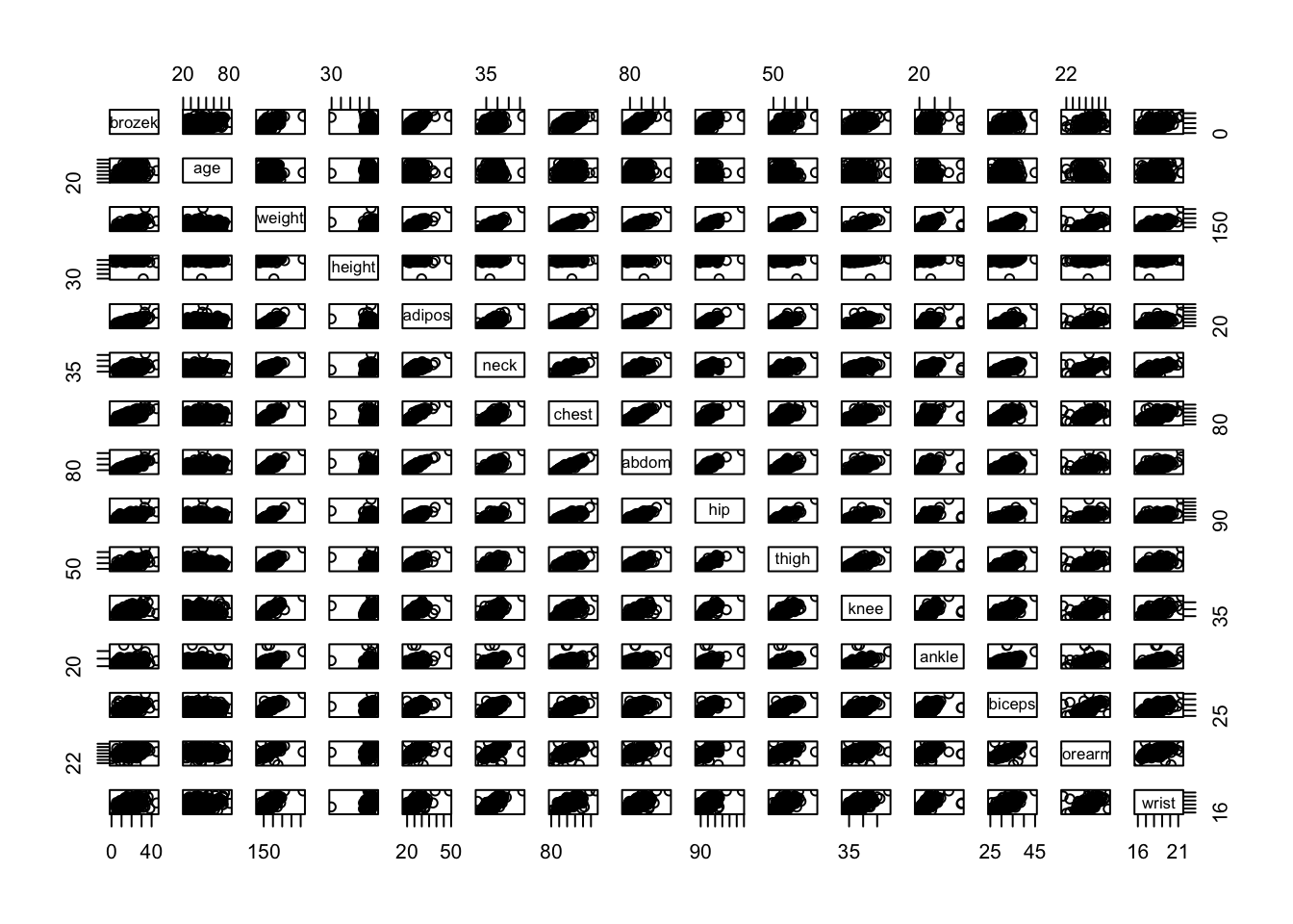
# (c)
# Add correlation coefficients
# Correlation panel

panel.cor <- function(x, y){
  usr <- par("usr"); on.exit(par(usr))
  par(usr = c(0, 1, 0, 1))
  r <- round(cor(x, y), digits=2)
  txt <- paste0(" ", r)
  text(0.5, 0.5, txt, cex = 0.8)
}
# Customize upper panel
upper.panel<-function(x, y){
  points(x,y, pch = 19)
}
# Create the plots
pairs(fat1,
      lower.panel = panel.cor,
      upper.panel = upper.panel)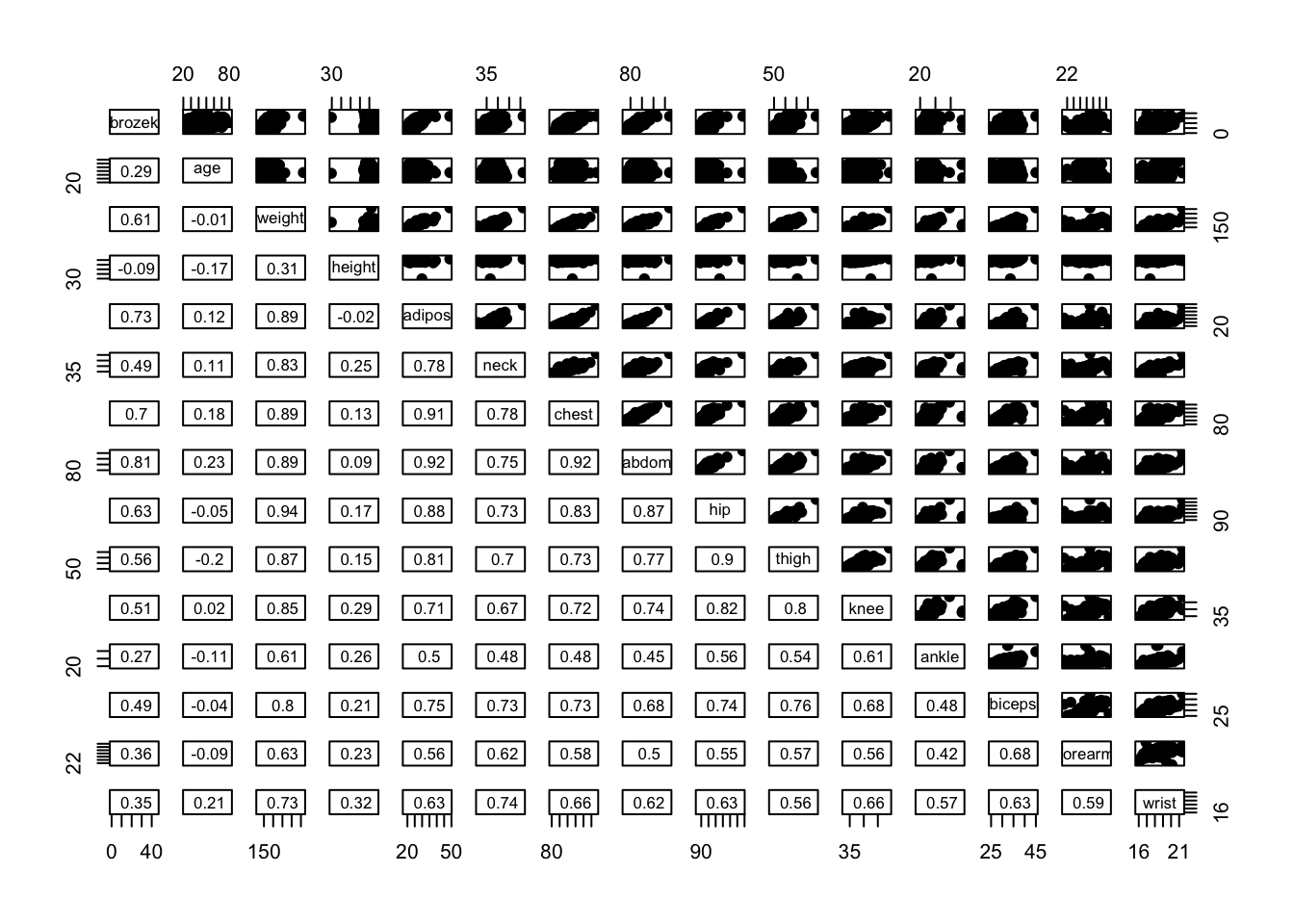
# A nicer plot  using the corrplot package.
#install.packages("corrplot")
library(corrplot)
## corrplot 0.92 loaded##
## Attaching package: 'corrplot'## The following object is masked from 'package:pls':
##
## corrplot#checking correlation between variables
corrplot(cor(fat1), method = "number", type = "upper", diag = FALSE)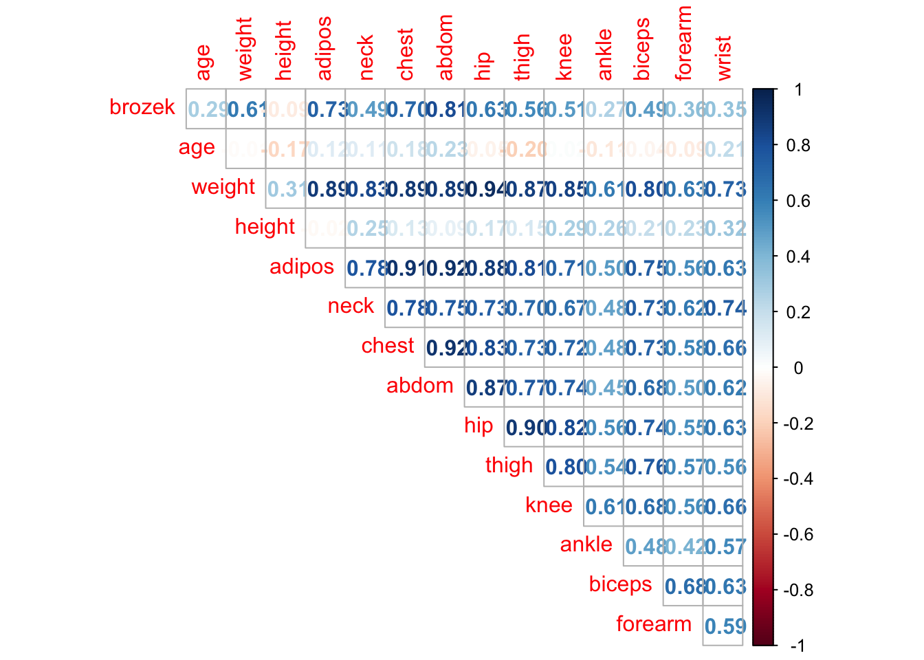
corrplot.mixed(cor(fat1), upper = "ellipse", lower = "number",number.cex = .7)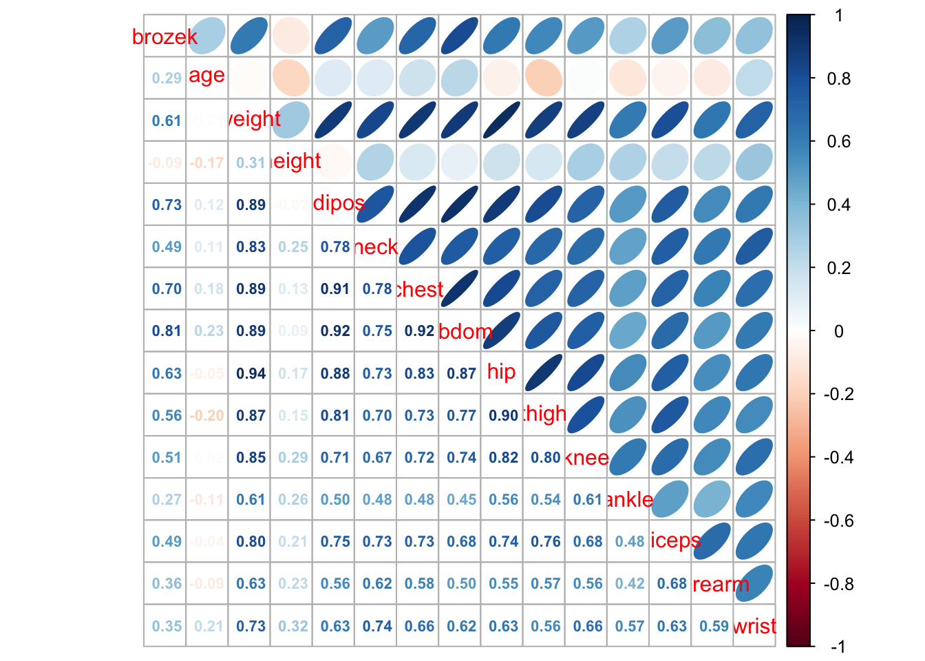
\(~\)
Simple Linear Regression
Following practical class 01, conduct simple linear regression modelling.
Linear regression model fitting
Exercise 2.2
- Use the
lm()function to fit a simple linear regression model, withbrozekas the response variable andadiposas the predictor variable. Save the result of the regression function toreg1. - Use
summary(reg1)command to get information about the model. This gives us the estimated coefficients, t-tests, p-values and standard errors as well as the R-square and F-statistic for the model. - Use
names(reg1)function to find what types of information are stored inreg1. For example, we can get or extract the estimated coefficients using the functioncoef(reg1)orreg1$coefficients.
Click for solution
## SOLUTION
# (a)
reg1 <- lm(brozek~adipos,data=fat1)

# (b)
summary(reg1)
##
## Call:
## lm(formula = brozek ~ adipos, data = fat1)
##
## Residuals:
## Min 1Q Median 3Q Max
## -21.4292 -3.4478 0.2113 3.8663 11.7826
##
## Coefficients:
## Estimate Std. Error t value Pr(>|t|)
## (Intercept) -20.40508 2.36723 -8.62 0.000000000000000778 ***
## adipos 1.54671 0.09212 16.79 < 0.0000000000000002 ***
## ---
## Signif. codes: 0 '***' 0.001 '**' 0.01 '*' 0.05 '.' 0.1 ' ' 1
##
## Residual standard error: 5.324 on 250 degrees of freedom
## Multiple R-squared: 0.53, Adjusted R-squared: 0.5281
## F-statistic: 281.9 on 1 and 250 DF, p-value: < 0.00000000000000022# (c)
names(reg1)## [1] "coefficients" "residuals" "effects" "rank"
## [5] "fitted.values" "assign" "qr" "df.residual"
## [9] "xlevels" "call" "terms" "model"coef(reg1)## (Intercept) adipos
## -20.405082 1.546712reg1$coefficients## (Intercept) adipos
## -20.405082 1.546712\(~\)
Confidence and prediction intervals
Exercise 2.3
- Obtain a \(95\%\) confidence interval for the coefficient estimates. Hint: use the
confint()command. - Obtain a \(95\%\) confidence and prediction intervals of
brozekfor a given value ofadipos. Assume this given value ofadiposis equal to 22.
Click for solution
## SOLUTION
# (a)
confint(reg1, level = 0.95)
## 2.5 % 97.5 %
## (Intercept) -25.067331 -15.74283
## adipos 1.365275 1.72815# (b)
newdata= data.frame(adipos=22)
predict(reg1,newdata=newdata, interval="confidence", level = 0.95)## fit lwr upr
## 1 13.62259 12.71416 14.53101predict(reg1,data.frame(adipos=22), interval="prediction", level = 0.95)## fit lwr upr
## 1 13.62259 3.096772 24.14841\(~\)
Regression diagnostics
Exercise 2.4
- Create a scatterplot of
adiposandbrozek. Is there a relationship between the two variables? - Plot
brozekandadiposalong with the least squares regression line using theplot()andabline()functions. - Use residual plots to check the assumptions of the model.
Click for solution
## SOLUTION
# (a) & (b)
plot(fat1$adipos, fat1$brozek, pch=16, col="cornflowerblue")
abline(reg1,lwd=3,col="red")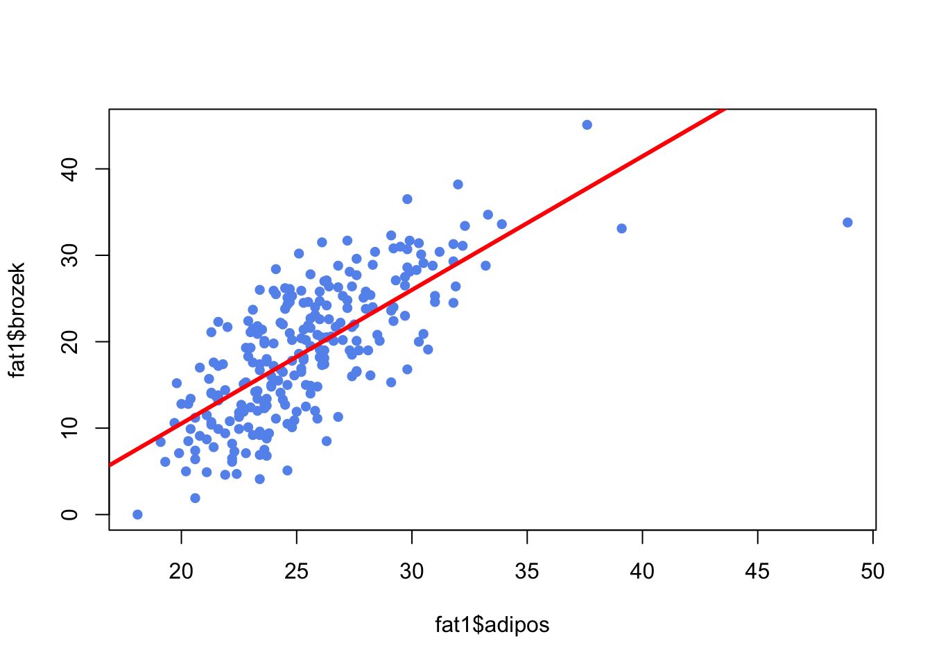
# (c)
par(mfrow=c(1,2)) # to have two plots side-by-side
plot(reg1, which=1,  pch=16, col="cornflowerblue")
plot(reg1, which=2,  pch=16, col="cornflowerblue")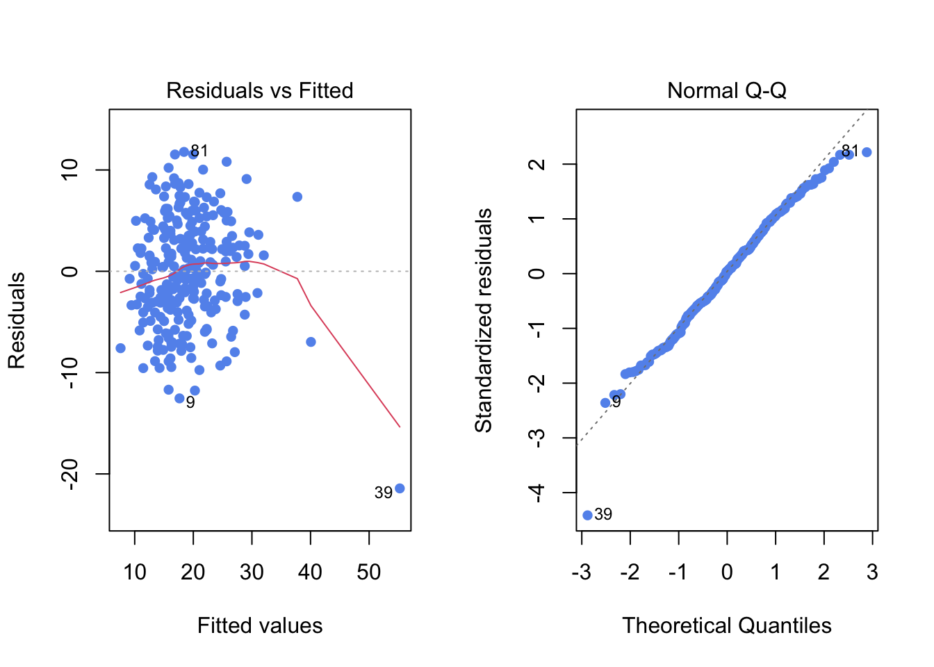
par(mfrow=c(1,1)) # to return to one plot per window \(~\)
Multiple Linear Regression
Linear regression model fitting
Exercise 2.5
- Use the
lm()function again to fit a linear regression model, withbrozekas the response variable and bothadiposandageas predictors. Save the result of the regression function toreg2. - Now use the
lm()function again to fit a linear regression model, withbrozekas the response variable and all other 14 variables as predictors. Save the result of the regression function toreg3. Hint: Uselm(brozek~., data=fat1). - Fit the same linear regression as in (b) but now exclude the age. Save the result of the regression function to
reg4. Hint: Uselm(brozek~.-age, data=fat1). - Compare the R-squares of these models. Notice we can extract the R-square value from the summary object as
summary(reg)$r.sq. Type?summary.lmto see what else is available. - Use Variance Inflation Factor (VIF) to assess if there is any relationship between the independent variables. Hint: use the
vif()function from thecarpackage.
Click for solution
## SOLUTION
# (a)
reg2 <- lm(brozek~adipos+age,data=fat1)
summary(reg2)
##
## Call:
## lm(formula = brozek ~ adipos + age, data = fat1)
##
## Residuals:
## Min 1Q Median 3Q Max
## -20.3523 -3.6914 -0.0805 3.5328 11.6982
##
## Coefficients:
## Estimate Std. Error t value Pr(>|t|)
## (Intercept) -24.75937 2.43119 -10.184 < 0.0000000000000002 ***
## adipos 1.49481 0.08875 16.842 < 0.0000000000000002 ***
## age 0.12643 0.02569 4.921 0.00000157 ***
## ---
## Signif. codes: 0 '***' 0.001 '**' 0.01 '*' 0.05 '.' 0.1 ' ' 1
##
## Residual standard error: 5.093 on 249 degrees of freedom
## Multiple R-squared: 0.5716, Adjusted R-squared: 0.5682
## F-statistic: 166.1 on 2 and 249 DF, p-value: < 0.00000000000000022# (b)
reg3 <- lm(brozek~.,data=fat1)
summary(reg3)##
## Call:
## lm(formula = brozek ~ ., data = fat1)
##
## Residuals:
## Min 1Q Median 3Q Max
## -10.2573 -2.5919 -0.1031 2.9040 9.2754
##
## Coefficients:
## Estimate Std. Error t value Pr(>|t|)
## (Intercept) -15.1901414 16.1089106 -0.943 0.3467
## age 0.0568795 0.0300278 1.894 0.0594 .
## weight -0.0813022 0.0498853 -1.630 0.1045
## height -0.0530707 0.1034409 -0.513 0.6084
## adipos 0.0610056 0.2779614 0.219 0.8265
## neck -0.4449644 0.2184007 -2.037 0.0427 *
## chest -0.0308670 0.0977939 -0.316 0.7526
## abdom 0.8789769 0.0854535 10.286 <0.0000000000000002 ***
## hip -0.2030661 0.1370728 -1.481 0.1398
## thigh 0.2273768 0.1355589 1.677 0.0948 .
## knee -0.0009927 0.2298076 -0.004 0.9966
## ankle 0.1572066 0.2075680 0.757 0.4496
## biceps 0.1485112 0.1600277 0.928 0.3543
## forearm 0.4296681 0.1848602 2.324 0.0210 *
## wrist -1.4792526 0.4966669 -2.978 0.0032 **
## ---
## Signif. codes: 0 '***' 0.001 '**' 0.01 '*' 0.05 '.' 0.1 ' ' 1
##
## Residual standard error: 3.996 on 237 degrees of freedom
## Multiple R-squared: 0.749, Adjusted R-squared: 0.7342
## F-statistic: 50.52 on 14 and 237 DF, p-value: < 0.00000000000000022# (c)
reg4 <- lm(brozek~.-age,data=fat1)
summary(reg4)##
## Call:
## lm(formula = brozek ~ . - age, data = fat1)
##
## Residuals:
## Min 1Q Median 3Q Max
## -9.5851 -2.7683 -0.0017 2.8892 9.0632
##
## Coefficients:
## Estimate Std. Error t value Pr(>|t|)
## (Intercept) -16.44809 16.18249 -1.016 0.3105
## weight -0.10069 0.04909 -2.051 0.0413 *
## height -0.07693 0.10323 -0.745 0.4568
## adipos 0.05355 0.27944 0.192 0.8482
## neck -0.40682 0.21865 -1.861 0.0640 .
## chest -0.02395 0.09826 -0.244 0.8076
## abdom 0.94825 0.07765 12.212 <0.0000000000000002 ***
## hip -0.22302 0.13741 -1.623 0.1059
## thigh 0.13510 0.12719 1.062 0.2892
## knee 0.10451 0.22417 0.466 0.6415
## ankle 0.11744 0.20762 0.566 0.5722
## biceps 0.17082 0.16046 1.065 0.2881
## forearm 0.37262 0.18338 2.032 0.0433 *
## wrist -1.15979 0.46969 -2.469 0.0142 *
## ---
## Signif. codes: 0 '***' 0.001 '**' 0.01 '*' 0.05 '.' 0.1 ' ' 1
##
## Residual standard error: 4.018 on 238 degrees of freedom
## Multiple R-squared: 0.7452, Adjusted R-squared: 0.7313
## F-statistic: 53.55 on 13 and 238 DF, p-value: < 0.00000000000000022# (d)
summary(reg1)$r.sq## [1] 0.5299755summary(reg2)$r.sq## [1] 0.5716312summary(reg3)$r.sq## [1] 0.7490309summary(reg4)$r.sq## [1] 0.7452313summary(reg4)$r.squared## [1] 0.7452313# or the adjusted R Squared
summary(reg4)$adj.r.squared## [1] 0.7313154# (e)
#install.packages("car") # you need to do this once
library(car)
vif(reg3)## age weight height adipos neck chest abdom hip
## 2.250902 33.786851 2.256593 16.163444 4.430734 10.684562 13.346689 15.158277
## thigh knee ankle biceps forearm wrist
## 7.961508 4.828828 1.945514 3.674508 2.193390 3.379612\(~\)
Interaction between variables (Additional)
It is straightforward to include the interaction between variables in the linear model using the lm() function. For example, the syntax chest*abdom will include chest, abdom and the interaction term chest x abdom as predictors.
summary(lm(brozek~chest*abdom, data=fat1))##
## Call:
## lm(formula = brozek ~ chest * abdom, data = fat1)
##
## Residuals:
## Min 1Q Median 3Q Max
## -9.9568 -3.2831 0.1953 2.8313 11.0567
##
## Coefficients:
## Estimate Std. Error t value Pr(>|t|)
## (Intercept) -95.206407 18.306007 -5.201 0.00000041538850 ***
## chest 0.404148 0.187669 2.154 0.032243 *
## abdom 1.498560 0.204429 7.330 0.00000000000323 ***
## chest:abdom -0.006936 0.001820 -3.810 0.000175 ***
## ---
## Signif. codes: 0 '***' 0.001 '**' 0.01 '*' 0.05 '.' 0.1 ' ' 1
##
## Residual standard error: 4.332 on 248 degrees of freedom
## Multiple R-squared: 0.6913, Adjusted R-squared: 0.6876
## F-statistic: 185.1 on 3 and 248 DF, p-value: < 0.00000000000000022We can also include a non-linear transformation of the predictors, using the function I(). For example, we can regress the response variable brozek on both adipos and adipos^2 as follows.
summary(lm(brozek~adipos+I(adipos^2), data=fat1))##
## Call:
## lm(formula = brozek ~ adipos + I(adipos^2), data = fat1)
##
## Residuals:
## Min 1Q Median 3Q Max
## -12.8991 -3.4058 -0.1397 3.7930 11.3518
##
## Coefficients:
## Estimate Std. Error t value Pr(>|t|)
## (Intercept) -55.688716 7.963036 -6.993 0.00000000002460 ***
## adipos 4.111738 0.561764 7.319 0.00000000000343 ***
## I(adipos^2) -0.045378 0.009814 -4.624 0.00000605491752 ***
## ---
## Signif. codes: 0 '***' 0.001 '**' 0.01 '*' 0.05 '.' 0.1 ' ' 1
##
## Residual standard error: 5.12 on 249 degrees of freedom
## Multiple R-squared: 0.5671, Adjusted R-squared: 0.5637
## F-statistic: 163.1 on 2 and 249 DF, p-value: < 0.00000000000000022We can also apply other transformations, e.g. taking the log of adipos.
summary(lm(brozek~log(adipos), data=fat1))##
## Call:
## lm(formula = brozek ~ log(adipos), data = fat1)
##
## Residuals:
## Min 1Q Median 3Q Max
## -13.5263 -3.3776 0.0751 3.8273 11.4306
##
## Coefficients:
## Estimate Std. Error t value Pr(>|t|)
## (Intercept) -119.233 7.813 -15.26 <0.0000000000000002 ***
## log(adipos) 42.820 2.419 17.70 <0.0000000000000002 ***
## ---
## Signif. codes: 0 '***' 0.001 '**' 0.01 '*' 0.05 '.' 0.1 ' ' 1
##
## Residual standard error: 5.174 on 250 degrees of freedom
## Multiple R-squared: 0.5562, Adjusted R-squared: 0.5544
## F-statistic: 313.3 on 1 and 250 DF, p-value: < 0.00000000000000022\(~\)
Variable Selection
Please review the practical demonstration 5.4) presented in the lecture.
Forward Stepwise Regression
Exercise 2.6
Use
regsubsets()to perform forward stepwise selection, assigning the result to a variable calledfwd. Note that you will need to (install and) load libraryleaps.Look at the summary of the resulting object
fwdand extract the following statistics for the model of each size: RSS, \(R^2\), \(C_p\), BIC and adjusted \(R^2\). Combine them into a single matrix.How many predictors are included in the models with i) minimum \(C_p\), ii) minimum BIC, and iii) maximum adjusted \(R^2\)? Which predictors are included in each case?
In a single plotting window, generate the following three plots, showing the relationship between the two variables as lines (as seen in the lecture practical demonstration 5.4): i) \(C_p\) against number of predictors, ii) BIC against number of predictors, and iii) adjusted \(R^2\) against number of predictors. Make sure to add relevant labels to the plots. Highlight the optimal model appropriately on each plot using a big red point.
Use the special
plot()function forregsubsetsto visualise the models obtained by \(C_p\).
Click for solution
## SOLUTION
# (a)
library("leaps") # required library for regsubsets() function.
fwd = regsubsets(brozek~., data = fat1, method = 'forward', nvmax = 14)

# (b)
results = summary(fwd)
results
## Subset selection object
## Call: regsubsets.formula(brozek ~ ., data = fat1, method = "forward",
## nvmax = 14)
## 14 Variables (and intercept)
## Forced in Forced out
## age FALSE FALSE
## weight FALSE FALSE
## height FALSE FALSE
## adipos FALSE FALSE
## neck FALSE FALSE
## chest FALSE FALSE
## abdom FALSE FALSE
## hip FALSE FALSE
## thigh FALSE FALSE
## knee FALSE FALSE
## ankle FALSE FALSE
## biceps FALSE FALSE
## forearm FALSE FALSE
## wrist FALSE FALSE
## 1 subsets of each size up to 14
## Selection Algorithm: forward
## age weight height adipos neck chest abdom hip thigh knee ankle biceps
## 1 ( 1 ) " " " " " " " " " " " " "*" " " " " " " " " " "
## 2 ( 1 ) " " "*" " " " " " " " " "*" " " " " " " " " " "
## 3 ( 1 ) " " "*" " " " " " " " " "*" " " " " " " " " " "
## 4 ( 1 ) " " "*" " " " " " " " " "*" " " " " " " " " " "
## 5 ( 1 ) " " "*" " " " " "*" " " "*" " " " " " " " " " "
## 6 ( 1 ) "*" "*" " " " " "*" " " "*" " " " " " " " " " "
## 7 ( 1 ) "*" "*" " " " " "*" " " "*" " " "*" " " " " " "
## 8 ( 1 ) "*" "*" " " " " "*" " " "*" "*" "*" " " " " " "
## 9 ( 1 ) "*" "*" " " " " "*" " " "*" "*" "*" " " " " "*"
## 10 ( 1 ) "*" "*" " " " " "*" " " "*" "*" "*" " " "*" "*"
## 11 ( 1 ) "*" "*" "*" " " "*" " " "*" "*" "*" " " "*" "*"
## 12 ( 1 ) "*" "*" "*" " " "*" "*" "*" "*" "*" " " "*" "*"
## 13 ( 1 ) "*" "*" "*" "*" "*" "*" "*" "*" "*" " " "*" "*"
## 14 ( 1 ) "*" "*" "*" "*" "*" "*" "*" "*" "*" "*" "*" "*"
## forearm wrist
## 1 ( 1 ) " " " "
## 2 ( 1 ) " " " "
## 3 ( 1 ) " " "*"
## 4 ( 1 ) "*" "*"
## 5 ( 1 ) "*" "*"
## 6 ( 1 ) "*" "*"
## 7 ( 1 ) "*" "*"
## 8 ( 1 ) "*" "*"
## 9 ( 1 ) "*" "*"
## 10 ( 1 ) "*" "*"
## 11 ( 1 ) "*" "*"
## 12 ( 1 ) "*" "*"
## 13 ( 1 ) "*" "*"
## 14 ( 1 ) "*" "*"RSS = results$rss
r2 = results$rsq
Cp = results$cp
BIC = results$bic
Adj_r2 = results$adjr2
# Combine the calculated criteria values above into a single matrix.
criteria_values <- cbind(RSS, r2, Cp, BIC, Adj_r2)
criteria_values## RSS r2 Cp BIC Adj_r2
## [1,] 5094.931 0.6621178 71.075501 -262.3758 0.6607663
## [2,] 4241.328 0.7187265 19.617727 -303.0555 0.7164672
## [3,] 4108.183 0.7275563 13.279341 -305.5638 0.7242606
## [4,] 3994.311 0.7351080 8.147986 -307.1180 0.7308182
## [5,] 3950.628 0.7380049 7.412297 -304.3597 0.7326798
## [6,] 3913.377 0.7404753 7.079431 -301.2177 0.7341196
## [7,] 3853.214 0.7444651 5.311670 -299.5925 0.7371342
## [8,] 3819.985 0.7466688 5.230664 -296.2456 0.7383287
## [9,] 3805.075 0.7476576 6.296894 -291.7018 0.7382730
## [10,] 3793.873 0.7484005 7.595324 -286.9153 0.7379607
## [11,] 3786.200 0.7489093 9.114827 -281.8960 0.7374010
## [12,] 3785.179 0.7489771 11.050872 -276.4346 0.7363734
## [13,] 3784.367 0.7490309 13.000019 -270.9592 0.7353225
## [14,] 3784.367 0.7490309 15.000000 -265.4298 0.7342058# (c)
which.min(Cp) # i) 8## [1] 8which.min(BIC) # ii) 4## [1] 4which.max(Adj_r2) # iii) 8## [1] 8coef(fwd, 4)## (Intercept) weight abdom forearm wrist
## -31.2967858 -0.1255654 0.9213725 0.4463824 -1.3917662# Looking at the summary above, the model with 4 predictors (minimum BIC)
# includes the predictors weight, abdom, forearm and wrist.
coef(fwd, 8)## (Intercept) age weight neck abdom hip
## -20.06213373 0.05921577 -0.08413521 -0.43189267 0.87720667 -0.18641032
## thigh forearm wrist
## 0.28644340 0.48254563 -1.40486912# The model with 8 predictors (minimum Cp and maximum adjusted R-squared)
# includes additionally the predictors age, neck, hip and thigh.
# (d)
par(mfrow = c(1, 3))
plot(Cp, xlab = "Number of Predictors", ylab = "Cp", type = 'l', lwd = 2)
points(8, Cp[8], col = "red", cex = 2, pch = 8, lwd = 2)
plot(BIC, xlab = "Number of Predictors", ylab = "BIC", type = 'l', lwd = 2)
points(4, BIC[4], col = "red", cex = 2, pch = 8, lwd = 2)
plot(Adj_r2, xlab = "Number of Predictors", ylab = "Adjusted RSq",
type = "l", lwd = 2)
points(8, Adj_r2[8], col = "red", cex = 2, pch = 8, lwd = 2)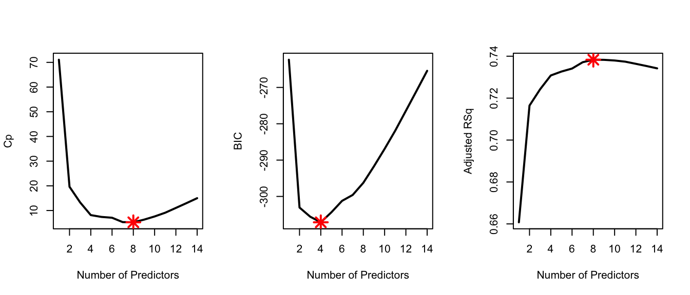
par(mfrow = c(1, 1))
plot(fwd, scale = "Cp")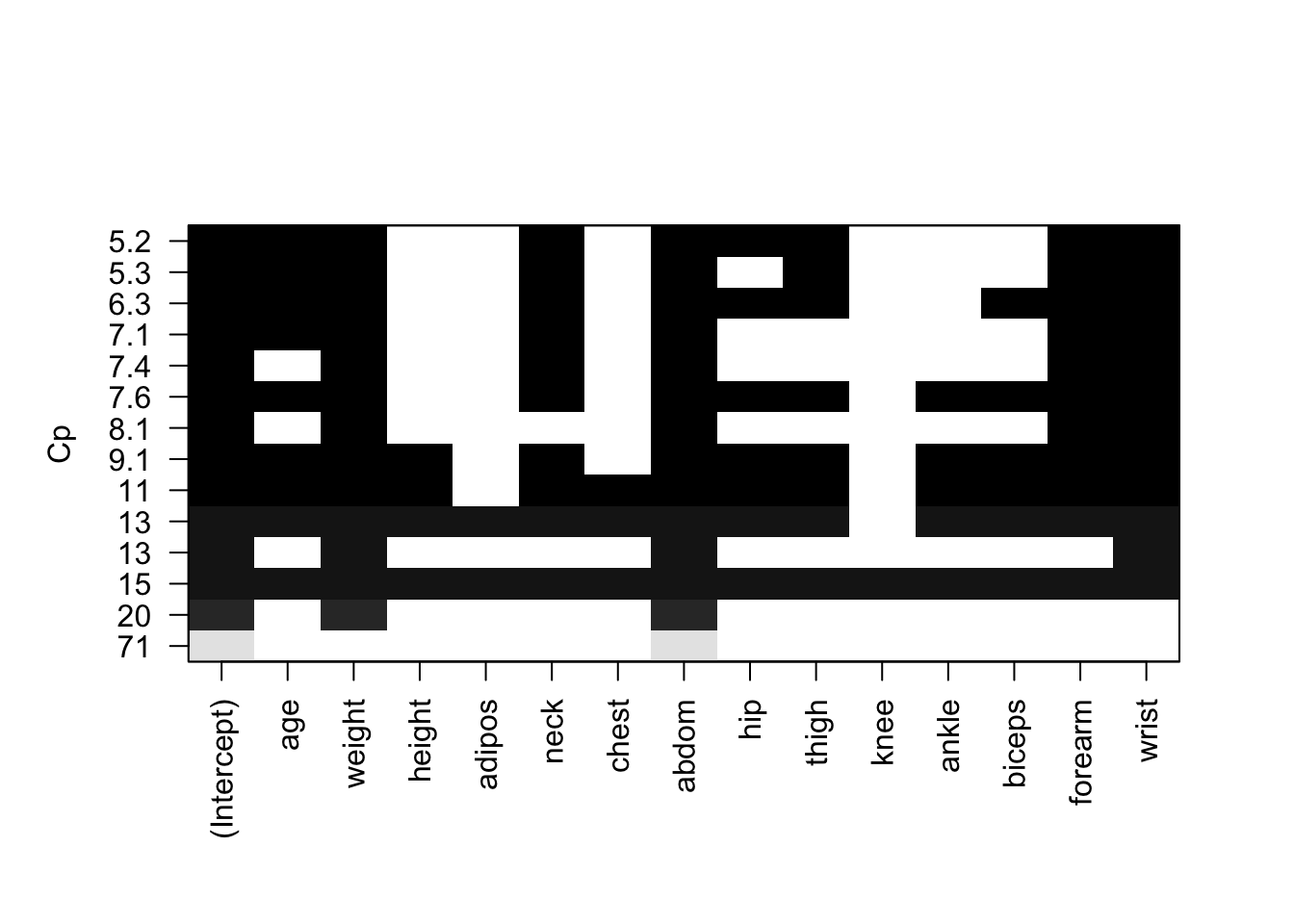
Best Subset and Backward Selection
Exercise 2.7
Do the best models (as determined by \(C_p\), BIC and adjusted-\(R^2\)) from best subset and backward stepwise selections have the same number of predictors? If yes, are the predictors the same as those from forward selection? Hint: if it is not obvious how to perform backward selection type ?regsubsets and see information about argument method.
Click for solution
## SOLUTION
best = regsubsets(brozek~., data = fat1, nvmax = 14)
bwd = regsubsets(brozek~., data = fat1, method = 'backward', nvmax = 14)

which.min(summary(best)$cp)
## [1] 8which.min(summary(best)$bic)## [1] 4which.max(summary(best)$adjr2)## [1] 8which.min(summary(bwd)$cp)## [1] 8which.min(summary(bwd)$bic)## [1] 4which.max(summary(bwd)$adjr2)## [1] 8# Yes, the three optimal models (under each of the criteria Cp, BIC and
# adj-R-squared) for each of forward stepwise, backward stepwise and
# best subset selections all have the same number of predictors.
# Cp
coef(fwd,8) ## (Intercept) age weight neck abdom hip
## -20.06213373 0.05921577 -0.08413521 -0.43189267 0.87720667 -0.18641032
## thigh forearm wrist
## 0.28644340 0.48254563 -1.40486912coef(best,8) ## (Intercept) age weight neck abdom hip
## -20.06213373 0.05921577 -0.08413521 -0.43189267 0.87720667 -0.18641032
## thigh forearm wrist
## 0.28644340 0.48254563 -1.40486912coef(bwd,8)## (Intercept) age weight neck abdom hip
## -20.06213373 0.05921577 -0.08413521 -0.43189267 0.87720667 -0.18641032
## thigh forearm wrist
## 0.28644340 0.48254563 -1.40486912# BIC
coef(fwd,4) ## (Intercept) weight abdom forearm wrist
## -31.2967858 -0.1255654 0.9213725 0.4463824 -1.3917662coef(best,4) ## (Intercept) weight abdom forearm wrist
## -31.2967858 -0.1255654 0.9213725 0.4463824 -1.3917662coef(bwd,4)## (Intercept) weight abdom forearm wrist
## -31.2967858 -0.1255654 0.9213725 0.4463824 -1.3917662# In addition, the predictors are also the same.
# adjusted R squared is not needed because it has also 8 predictors