Chapter 11 Generalised Additive Models
11.1 Review
- We started with polynomial regression, which is a flexible smoother but is global and therefore overall sensitive to changes in the data.
- Then we considered regression based on step functions, which has the advantage of being local, but is not smooth.
- We have introduced piecewise polynomials. These achieve local smoothness, but can result in strange-looking discontinuous curves.
- We started to add constraints, which ensure continuity and smoothness, leading to more modern methods like cubic splines and natural splines.
- Finally, we discussed smoothing splines, which are continuous non-linear smoothers that bypass the problem of knot selection altogether.
All the non-linear models we have seen so far
- Global Polynomials
- Step Functions
- Regression Splines
- Natural Splines
- Smoothing Splines
take as input one predictor and utilise suitable transformations of the predictor (namely powers) to produce flexible curves that fit data that exhibit non-linearities.
This final chapter covers the case of multiple predictors!
11.2 GAMs
A Generalised Additive Model (GAM) is an extension of the multiple linear model, which recall is \[ y= \beta_0 + \beta_1x_1 + \beta_2x_2 + \ldots + \beta_p x_p +\epsilon. \] In order to allow for non-linear effects a GAM replaces each linear component \(\beta_jx_j\) with a non-linear function \(f_j(x_j)\).
So, in this case we have the following general formula \[ y= \beta_0 + f_1(x_1) + f_2(x_2) + \ldots + f_p(x_p) +\epsilon. \] This is called an additive model because we estimate each \(f_j(x_j)\) for \(j = 1,\ldots,p\) and then add together all of these individual contributions.
Backfitting algorithm
A simple iterative procedure, backfitting algorithm, can be used to fit the model.
- We set \(\hat{\beta}_0=\bar{y}\), and it never changes.
- For each predictor \(j\), fit the function \(\hat{f}_j\) to \(\{y_i-\hat{\beta}_0-\sum_{k\neq j} \hat{f}_k(x_{ik})\}_{i=1}^{n}\) using the current estimates of the other functions \(\hat{f}_k\).
- Continue the process until the estimates \(\hat{f}_j\) stabilize.
Flexibility
Note that because we can have a different function \(f_j\) for each \(X_j\), GAMs are extremely flexible. So, for example a GAM may include:
- Any kind of non-linear polynomial method from the ones we have seen for continuous predictors.
- Step functions which are more appropriate for categorical predictors.
- Linear models if that seems more appropriate for some predictors.
Example: Wage Data
GAMs are very useful as they estimate the contribution of the effects of each predictor.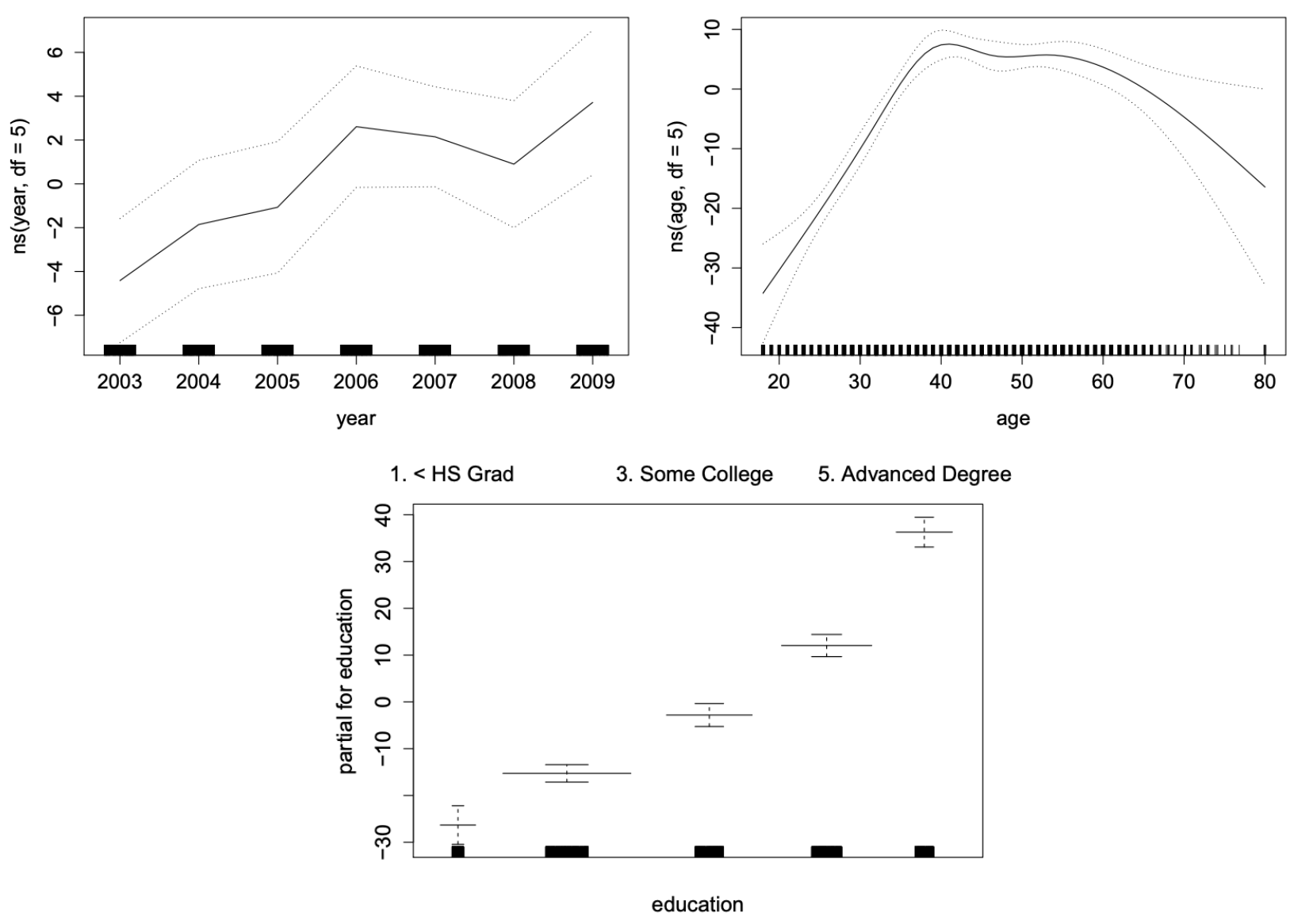
Figure 11.1: GAM using cubic splines for year and age, and step functions for education (which is categorical).
Pros and Cons
Pros:
- Very flexible in choosing non-linear models and generalisable to different types of responses.
- Because of the additivity we can still interpret the contribution of each predictor while considering the other predictors fixed.
- GAMs can outperform linear models in terms of prediction.
Cons:
- Additivity is convenient but it is also one of the main limitations of GAMs.
- GAMs might miss non-linear interactions among predictors. Of course, we can add manually interaction terms but ideally we would prefer a procedure which does that automatically.
11.3 Practical Demonstration
In this final part we will fit a generalised additive model (GAM) utilising more than one predictor from the Boston dataset.
library(MASS)
y = Boston$medv
x = Boston$lstat
y.lab = 'Median Property Value'
x.lab = 'Lower Status (%)'
We first use the command names() in order to check once again the available predictor variables.
names(Boston)## [1] "crim" "zn" "indus" "chas" "nox" "rm" "age"
## [8] "dis" "rad" "tax" "ptratio" "black" "lstat" "medv"Let’s say that we want to use predictors lstat, indus and chas for the analysis (use ?Boston again to check what these refer to).
For GAMs we will make use of the library gam in RStudio, so the first thing that we have to do is to install this package by executing install.packages("gam") once. Then we load the library.
library(gam)## Loading required package: foreach## Loaded gam 1.20The main function is gam(). Inside this function we can use any combination of non-linear and linear modelling of the various predictors. For, example below we use a cubic spline with 3 degrees of freedom for lstat, a smoothing spline with 3 degrees of freedom for indus and a simple linear model for variable chas. We then plot the contributions of each predictor using the command plot(). As we can see, GAMs are very useful as they estimate the contribution of the effects of each predictor.
gam = gam( medv ~ bs(lstat, degree = 3, df = 5) + s(indus, df = 5) + chas,
           data = Boston )
par( mfrow = c(1,3) )
plot( gam,  se = TRUE, col = "blue" )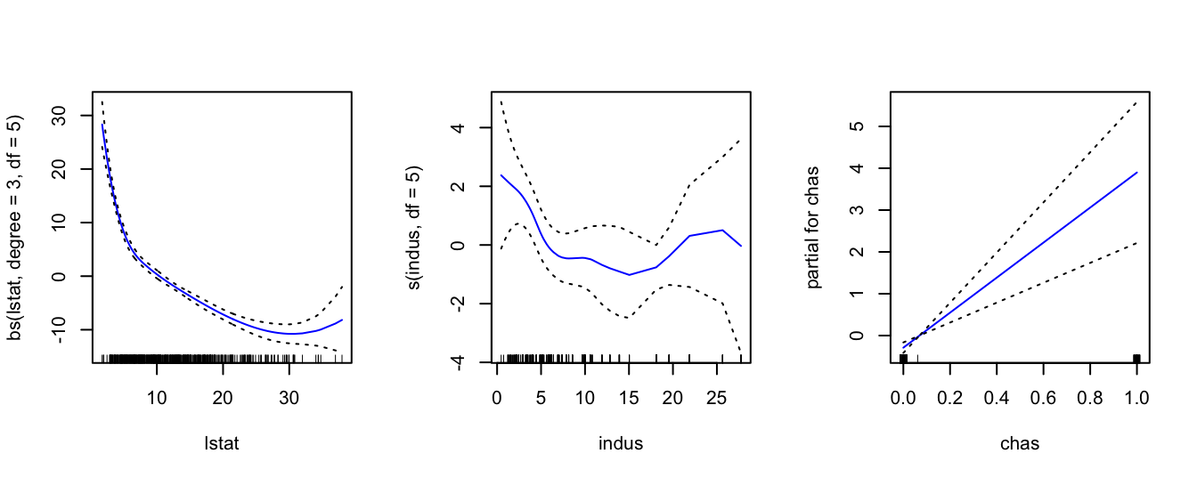
Note that simply using chas inside gam() is just fitting a linear model for this variable. However, one thing that we observe is that variable is binary as it only takes the values of 0 and 1. This we can see from the x-axis of the chas plot on the right above. So, it would be preferable to use a step function for this variable. In order to do this we have to change the variable chas to a factor. We first create a second object called Boston1 (in order not to change the initial dataset Boston) and then we use the command factor() to change variable chas. Then we fit again the same model. As we can see below now gam() fitted a step function for variable chas which is more appropriate.
Boston1 = Boston
Boston1$chas = factor(Boston1$chas)

gam1 = gam( medv ~ bs(lstat, degree = 3, df = 5) + s(indus, df = 5) + chas,
            data = Boston1 )
par(mfrow = c(1,3))
plot(gam1,  se = TRUE, col = "blue")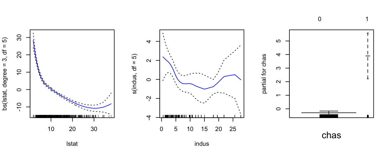
We can make predictions from gam objects, just like lm objects, using the predict() method for the class gam. Here we make predictions on some new data. Note that when assigning the value 0 to chas, we enclose it in "" since we informed R to treat chas as a categorical factor with two levels - "0" and "1".
preds <- predict( gam1,
                  newdata = data.frame( chas = "0", indus = 3, lstat = 5 )  )
preds
## 1
## 32.10065