18 Logistic Regression
18.1 Concepts
The last chapter covered a few things we shouldn’t do in an OLS regression. One additional thing we should not do is use either a categorical or a dichotomous variable as the dependent variable. Why? Let’s look at that visually, using a variable that has the values 0 and 1.
Let’s look at the data that we’ve used to estimate wages in the past, and let’s make occupation a numeric variable, with 1 being white collar workers and 0 being blue collar workers. Let’s see whether higher levels of education predict that an individual will be a white collar worker, rather than a blue collar worker.
##
## Call:
## lm(formula = occnum ~ education, data = PSID1982)
##
## Residuals:
##      Min       1Q   Median       3Q      Max
## -0.96527 -0.39016  0.03473  0.18496  1.18496
##
## Coefficients:
##              Estimate Std. Error t value Pr(>|t|)
## (Intercept) -0.990119   0.074246  -13.34   <2e-16 ***
## education    0.115023   0.005648   20.36   <2e-16 ***
## ---
## Signif. codes:  0 '***' 0.001 '**' 0.01 '*' 0.05 '.' 0.1 ' ' 1
##
## Residual standard error: 0.3841 on 593 degrees of freedom
## Multiple R-squared:  0.4115, Adjusted R-squared:  0.4105
## F-statistic: 414.7 on 1 and 593 DF,  p-value: < 2.2e-16
The linear regression results seem to indicate that yes, individuals with more education tend to be white collar workers. But an OLS regression isn’t really an appropriate way to answer that question, and it’s pretty easy to see why if we look at a graph of the two variables.
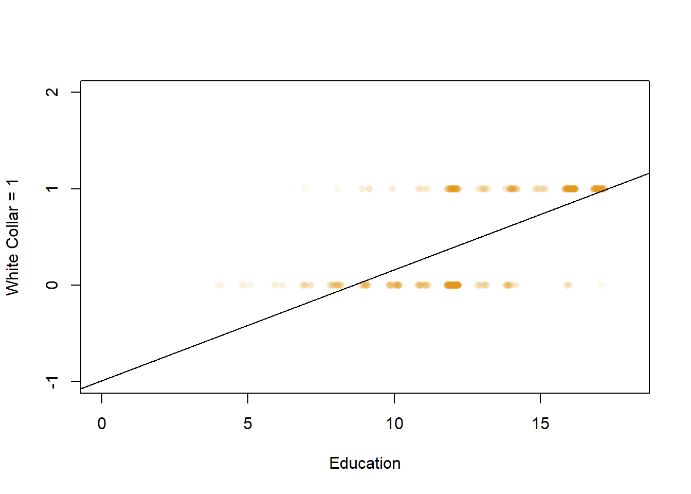
Pardon my French, but wtf is that graph telling me? The line shows me that people who are more educated tended to be white collar workers, just like the regression output above. And the slope for that line matches the number of the coefficient we calculated with the regression above. And the point x=0 is just below -1, which is the constant for the regression above. But what does it mean to be -.99 for white collar worker? Being a white collar worker is either a yes or a no, a person either is a white collar or a blue collar worker. They don’t work as a white collar worker in this data a little bit or marginally, it’s an act that is either done or not done.
And notice that the straight line we generated ventures below 0 and continues to the right of the graph indefinitely. Eventually it’ll cross the value 2 for white collar worker, which equals what exactly? A 1 on white collar work is as high as the data allows, we can’t say that’s a “double white collar worker”. That’s all to say that fitting a straight line is inappropriate here. Our outcome variable only has two values, so we don’t want to our regression to give us values that are impossible.
That’s the intuition for why linear regression isn’t always the best tool for estimating the relationship for every dependent variable. This section will explain one alternative we can use in the case that we have a dichotomous dependent variable that only takes two values (yes/no, 0/1, on/off, voted/didn’t vote, etc.).
18.1.1 Logistic regression
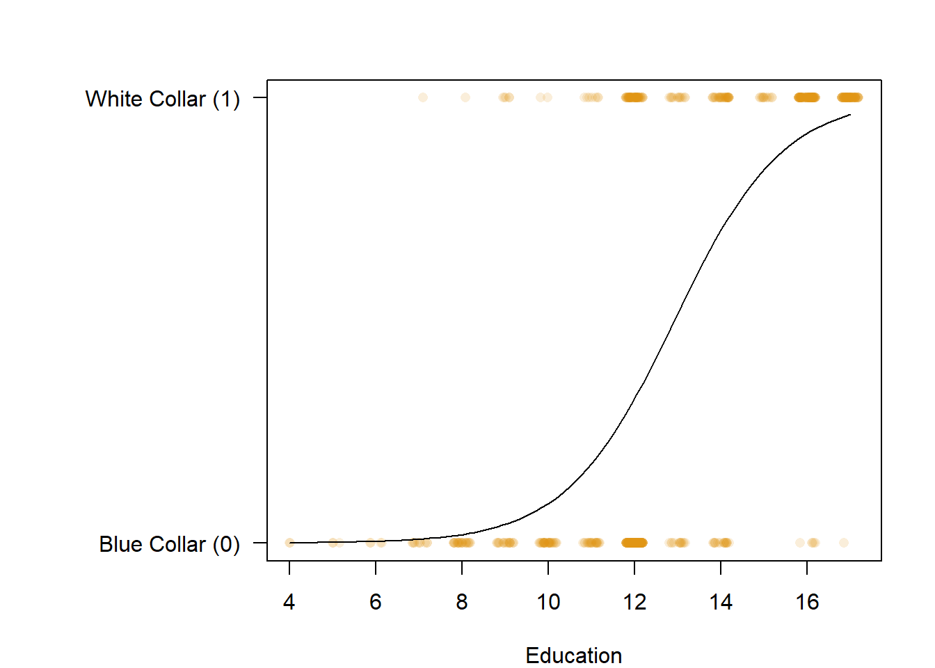
Also known as logit regression, Logistic regression is a strategy for estimating the probability of a dichotomous outcome. For instance, either an event happening or not happening or a person doing either one thing or another. Rather than using a linear line to estimate the relationship between the independent and dependent variable, as we did above, logistic regression uses a “s” shaped curve.
What the linear regression is doing at it’s most basic is calculating the mean of our dependent variable for all of the different values in our independent variable(s). So when we look at the wages of people as a result of their education, it looks at the average wages for someone with 4 years of education, and 5 years of education, and 6 years of education, and on up and see whether those averages increase or decrease as our independent variable increases.
Logistic regression works a little different. What it is doing is looking at the probability that the dependent variable is in one group or another (yes or no, 0 or 1, white collar or blue collar), as the independent variable changes. So, let’s look above, and try to intuit that a bit. What is the probability that someone is a white collar worker at the lowest value of education (a 4)? 0, no one with that little education is a white collar worker. What about at 5? Most likely the person is a blue collar worker still. And up and up. What about at 17, the highest value for education? The probability is pretty high that they’re a white collar worker. The logistic regression is trying to figure out which of two groups an observation falls into based on changes in our independent variable. For some it will be wrong. There are people with a 7 on education that would be predicted to be blue collar workers in the above model, but they’re still white collar workers. What the logistic regression does is try to minimize those errors.
Let’s talk about interpreting a linear regression. Linear regression gives us coefficients that are in the units of our dependent variable, so we could say that a one unit increase in education would be associated with $X increase in wages for an individual. With a logistic regression, we want to describe the impact of our independent variable(s) on the probability of being in one of two groups. Specifically, the coefficients we are provided by default by R are the log-odds, which are the logarithm of the odds \({\frac{p}{1-p}}\) where p is a probability. I’m going to go into more detail on all of that below, but for now let’s work through interpreting the regression we ran above. Here are the logistic regression results for the relationship of education on the probability that a worker was white collar.
##
## Call:
## glm(formula = occupation ~ education, family = binomial, data = PSID1982)
##
## Deviance Residuals:
##      Min        1Q    Median        3Q       Max
## -2.56065  -0.88470  -0.08998   0.40788   3.07286
##
## Coefficients:
##              Estimate Std. Error z value Pr(>|z|)
## (Intercept) -10.27892    0.84276  -12.20   <2e-16 ***
## education     0.79523    0.06589   12.07   <2e-16 ***
## ---
## Signif. codes:  0 '***' 0.001 '**' 0.01 '*' 0.05 '.' 0.1 ' ' 1
##
## (Dispersion parameter for binomial family taken to be 1)
##
##     Null deviance: 824.47  on 594  degrees of freedom
## Residual deviance: 511.84  on 593  degrees of freedom
## AIC: 515.84
##
## Number of Fisher Scoring iterations: 5
For each one unit increase in education, the log-odds for being a white collar worker increase by .795, and that change is significant. That isn’t too different from how we would interpret a linear regression, but we need to be specific in stating that it is the log-odds that have changed.
18.1.2 Predictions
It’s useful to think about how we can use logistic regression, Whereas in linear regression we would predict a specific wage for each level of education, here we would predict a certain probability that each level of education would be in a given occupation (white collar or blue collar). Just as we could create a prediction for the specific wage given an education level using the coefficient for our regression, we can make a similar calculation using our logistic results.
Probabilities run from 0 to 1. In the case of this regression, a probability of 0 would mean there is 0 chance a person with that level of education would be a white collar worker, and a probability of 1 would mean we’re absolutely certain that person is a white collar worker. In general though, logistic regressions rarely give us probabilities of 0 or 1, because there is often still a small chance of either outcome happening.
We can calculate the specific probability for any level of education using our coefficient and this formula, where p(x) is the probability of any value (x) of our independent variable being classified a 1 (white collar worker), and e stands for taking the exponent (you can take the exponent in r using exp()).
p(x) = \(\frac{e^{\beta_{0} + \beta X_{1}}}{1 + e^{\beta_{0} + \beta X_{1}}}\)
And so we can calculate using that formula and the coefficient from the regression above, which was .79. The lowest value in education was 4 and the highest was 17, so let’s calculate it for two numbers in the middle (8 and 15).
p(8) = \(\frac{e^{-10.27892 + 8*0.79523}}{1 + e^{-10.27892 + 8*0.79523}}\) = \(\frac{e^{-3.91708}}{1 + e^{-3.91708}}\) = 0.01951087
p(15) = \(\frac{e^{-10.27892 + 15*0.79523}}{1 + e^{-10.27892 + 15*0.79523}}\) = \(\frac{e^{1.64953}}{1 + e^{1.64953}}\) = 0.8388275
The model thinks that someone with 8 years of education has a very low probability of working a white collar job, but thinks a person with 15 years would be very likely to.
We can see all the specific predicted classifications based on education below.
## education probabilities prediction
## 1 4 0.0008260888 blue pred
## 2 5 0.0018279180 blue pred
## 3 6 0.0040397911 blue pred
## 4 7 0.0089042667 blue pred
## 5 8 0.0195115015 blue pred
## 6 9 0.0422164022 blue pred
## 7 10 0.0889454691 blue pred
## 8 11 0.1777969058 blue pred
## 9 12 0.3238549802 blue pred
## 10 13 0.5147761977 white pred
## 11 14 0.7014800651 white pred
## 12 15 0.8388355664 white pred
## 13 16 0.9201820630 white pred
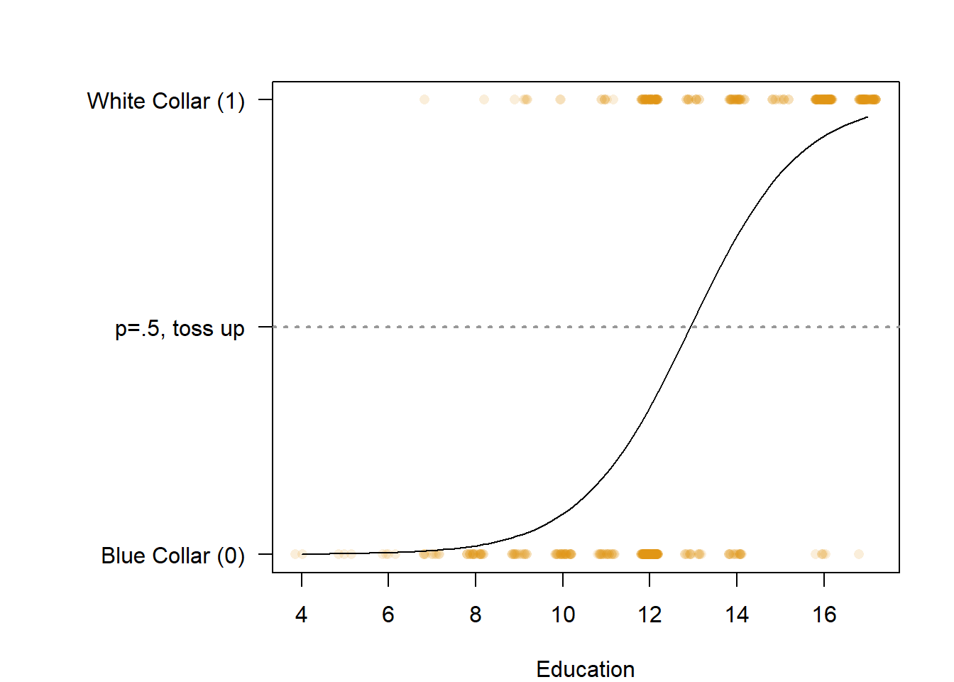
## 14 17 0.9623141786 white predBy default, any row that the model predicts with less than a .5 probability of being in class 1, is assigned to class 0. and any row that it predicts to have a .5 probability or above of being in class 1, is assigned to class 1. We can adjust that, but I’ve never done that, so I don’t even know how and I wouldn’t recommend doing it unless you’re sure it’s the right thing to do. Just saying it’s possible.
We can also visualize that p=.5 cutoff point using our graph above.
18.1.3 Error Rates
Above, 9 of the 17 levels of education were predicted to be blue collar workers, and 58% of workers as a result were predicted to be blue collar. How do we evaluate that prediction? There are ways that we can evaluate the strength of our regression model and the predictions classifications it made. Let’s start by evaluating it’s predictions.
58% of workers were predicted to be blue collar, but only 51.2% of workers were actually blue collar. Uh oh, that means that some people were wrongly predicted to be blue collar, and the opposite is probably true too, some workers that are blue collar were predicted to be white collar. We can think about that as the error rate for our logistic regression model.
We can calculate the error rate by taking the wrong guesses from our model and dividing it by the total number of guesses. Typically, these are thought of as positive and negative tests. It comes from the medical literature, where they’re very concerned with whether a medical tests gives people a false positive, saying they have a disease when they don’t, and false negatives, telling a person they don’t have a disease when they really do. True positives and true negatives are good, but false positives and negatives can have really delirious effects on people. Anyways, that’s to explain why the formula for the error rate discusses positives and negatives, when our results are white and blue collar. You can think of the false positives being times the model predicted a blue collar worker was a white collar worker, and false negatives being predicted white collar workers that are actually blue collar.
| blue pred | white pred | |
|---|---|---|
| blue real | 269 | 36 |
| white real | 76 | 214 |
So above, workers that are blue collar are labeled “blue real”, while those that were predicted to be blue collar are labeled “blue pred”. As such, 269 workers that are blue collar were predicted to be blue collar. Those are “true negatives” in this case. 214 workers that are white collar (“white real”) had correct predictions in the data, those are true positives. 36 were false positives, and 76 were false negatives. So what’s the error rate then?
error rate = false positives + false negatives/ true positives+ true negatives + false positives + false negatives = (76+36)/(269+214+76+36) = 0.1882353 = 18.8%. So the model was wrong on roughly 19% of cases. That’s not great. You wouldn’t trust a medical test very much if it was going to be wrong 19% of the time.
The inverse of the error rate is the accuracy rate. You can calculate the accuracy rate by subtracting 1 by the fraction of wrong guesses (or 100 minus the error rate as a percentage). Alternatively, you can look at the share of correct guesses (true positive and true negative) divided by the total number of predictions. Here that would be 1-0.1882353, which equals .8117647 or 81.2%.
We have two other measures we like to use as part of our evaluation of how correct the predictions are. Sensitivity measures the share of true postiives that the model predicts relative to the number of positives in the data. Essentially, it measures how well the model performed in cases it labeled as the “positive case”, or white collar in this situation. To state that yet another way, it measures the percentage of white collar workers that the model predicted would be white collar workers.
sensitivity = true positives/(true positives+ false negatives) = 214/ (214+76) = 0.737931 = 73%
On the other hand, the specificity measures how well the model performed at predicting the negative case or blue collar workers. Similarly, we divide the number of true negatives in our data, by the number of true negatives and false positives.
specificity = true negative/(true negative + false positive) = 269/(269+36) =0.8819672 = 88%.
So the model did a better job of predicting the occupation blue collar workers correctly than white collar workers using only education.
We can also evaluate whether the model would have done better just making predictions without any independent variables. Let me explain what I mean. If you knew that 51.2% of workers in the data were blue collar workers, and I told you to predict the occupation of a random worker, what would you guess? The best bet would be to say they were a blue collar worker, because you’ll be right more than you’ll be wrong. You might only be right 51.2% of the time, but you’d only be right. 48.8% of the time if you guessed white collar worker for everyone. So, at minimum we should ask that our model improves our prediction making, which isn’t always the case. That can be particularly difficult when our dependent variable is heavily imbalanced. For instance, say that our data was 95% blue collar workers and only 5% white collar. We’d get 95% of guesses right just by predicting blue collar for everyone, so it becomes more difficult for our model to make our predictions better. Not impossible, just more difficult.
18.1.4 Other Metrics for Evaluation
There are also more statistically intensive ways of evaluating our model. Let’s go back to our output.
##
## Call:
## glm(formula = occnum ~ education, family = binomial, data = PSID1982)
##
## Deviance Residuals:
##      Min        1Q    Median        3Q       Max
## -2.56065  -0.88470  -0.08998   0.40788   3.07286
##
## Coefficients:
##              Estimate Std. Error z value Pr(>|z|)
## (Intercept) -10.27892    0.84276  -12.20   <2e-16 ***
## education     0.79523    0.06589   12.07   <2e-16 ***
## ---
## Signif. codes:  0 '***' 0.001 '**' 0.01 '*' 0.05 '.' 0.1 ' ' 1
##
## (Dispersion parameter for binomial family taken to be 1)
##
##     Null deviance: 824.47  on 594  degrees of freedom
## Residual deviance: 511.84  on 593  degrees of freedom
## AIC: 515.84
##
## Number of Fisher Scoring iterations: 5
A lot is the same as from our linear regression output, but we no longer have an r-squared or adjusted r-squared. That’s because we can’t calculate the sums of the squared errors the same way for a logistic regression. However, there are alternative methods. Actually, there are a lot. Researchers and statisticians keep developing new formulas to evaluate logistic regression models, but non have quite replaced R-Squared, in part because none are as simple to understand. And actually, I’ve shied away form using what are called pseudo R-Squared’s because no one really understands what they measure. You can read a good description of some of the issues here from The Stats Geek if you’re interested. But I decided not to explain it here.
The good news is we should recognize one metric at the bottom of our table: AIC. AIC can be calculated for logistic regression models, and can be used to evaluate the overall goodness-of-fit for the regression and in determining whether independent variables should be included.
Long story short, when you’re evaluating your models look at it’s error rate, look at the error rate if you didn’t include any independent variables, and use AIC.
18.1.5 Multiple Independent Variables
Running a logistic regression with multiple independent variables isn’t too different.
##
## Call:
## glm(formula = occnum ~ education + gender + ethnicity, family = binomial,
##     data = PSID1982)
##
## Deviance Residuals:
##      Min        1Q    Median        3Q       Max
## -2.54411  -0.85360  -0.08406   0.41824   3.11388
##
## Coefficients:
##                Estimate Std. Error z value Pr(>|z|)
## (Intercept)    -9.86521    0.90222 -10.934   <2e-16 ***
## education       0.80364    0.06696  12.002   <2e-16 ***
## gendermale     -0.71189    0.34305  -2.075    0.038 *
## ethnicityother  0.11137    0.41885   0.266    0.790
## ---
## Signif. codes:  0 '***' 0.001 '**' 0.01 '*' 0.05 '.' 0.1 ' ' 1
##
## (Dispersion parameter for binomial family taken to be 1)
##
##     Null deviance: 824.47  on 594  degrees of freedom
## Residual deviance: 507.45  on 591  degrees of freedom
## AIC: 515.45
##
## Number of Fisher Scoring iterations: 5
Each one unit increase in education is associated with a .80 increase in the log-odds of being a white collar worker when holding gender and ethnicity constant, and that change is significant.
Being female, rather than male, is associated with log-odds that are .71 higher for being a white collar worker, holding ethnicity and education constant, and that change is significant.
Being African American, rather than other ethnicities, is associated with log-odds that are .11 lower for being a white collar worker, holding education and gender constant, and that change is insignificant.
18.2 Practice
Let’s work through an example using some data on volunteering, which has information on individuals and how neurotic they are, how extroverted they are, their gender, and whether they volunteered. The data was collected to help understand the personalities of people that volunteer. The variable for volunteering was originally coded as a yes/no, and we’ll turn that into a numeric variable with the value of 1 if the individual volunteered. We’ll use volunteering as the dependent variable, and we’ll include all the other variables as independent variables eventually. Let’s start with neuroticism.
To run the regression below we need to change to things from our usual line of code for a regression. We can’t use the command lm(), because lm is for linear models. Instead, we want to use the command glm(), which stands for generalized linear models. Essentially, it allows us to adjust the linear model in a few different ways, most of which we don’t need to worry about right now. We can run different types of models using the glm() command though, so we also need to add the option family at the end of our command, and set that to binomial.
Cowles <- read.csv("https://raw.githubusercontent.com/ejvanholm/DataProjects/master/Cowles.csv")
summary(glm(volunteer~neuroticism, data=Cowles, family=binomial))
##
## Call:
## glm(formula = volunteer ~ neuroticism, family = binomial, data = Cowles)
##
## Deviance Residuals:
## Min 1Q Median 3Q Max
## -1.068 -1.045 -1.032 1.313 1.343
##
## Coefficients:
## Estimate Std. Error z value Pr(>|z|)
## (Intercept) -0.382202 0.137090 -2.788 0.0053 **
## neuroticism 0.005222 0.010976 0.476 0.6342
## ---
## Signif. codes: 0 '***' 0.001 '**' 0.01 '*' 0.05 '.' 0.1 ' ' 1
##
## (Dispersion parameter for binomial family taken to be 1)
##
## Null deviance: 1933.5 on 1420 degrees of freedom
## Residual deviance: 1933.3 on 1419 degrees of freedom
## AIC: 1937.3
##
## Number of Fisher Scoring iterations: 4A one unit increase in neuroticism is associated with a .005 increase in the log-odds that someone volunteered, but that change is insignificant.
##
## Call:
## glm(formula = volunteer ~ neuroticism + extraversion + sex, family = binomial,
##     data = Cowles)
##
## Deviance Residuals:
##     Min       1Q   Median       3Q      Max
## -1.3977  -1.0454  -0.9084   1.2601   1.6849
##
## Coefficients:
##               Estimate Std. Error z value   Pr(>|z|)
## (Intercept)  -1.116496   0.249057  -4.483 0.00000736 ***
## neuroticism   0.006362   0.011357   0.560     0.5754
## extraversion  0.066325   0.014260   4.651 0.00000330 ***
## sexmale      -0.235161   0.111185  -2.115     0.0344 *
## ---
## Signif. codes:  0 '***' 0.001 '**' 0.01 '*' 0.05 '.' 0.1 ' ' 1
##
## (Dispersion parameter for binomial family taken to be 1)
##
##     Null deviance: 1933.5  on 1420  degrees of freedom
## Residual deviance: 1906.1  on 1417  degrees of freedom
## AIC: 1914.1
##
## Number of Fisher Scoring iterations: 4
A one unit change in neuroticism is associated with a .006 increase in the log-odds that they volunteered, holding their extroversion and sex constant, and that change is insignificant.
A one unit change in extroversion is associated with a .066 increase in the log-odds that they volunteered, holding their neuroticism and sex constant, and that change is significant.
Being a male, as opposed to a female, is associated with a .24 decrease in the log-odds that they volunteered, holding their neuroticism and extroversion constant, and that change is significant.
That’s really the only line of code we need to practice from this chapter! But, it’s a big line, because anytime you want to run a regression with a dichotomous dependent variable that is the correct form.
Let’s look at some of the evaluation techniques described above. First, what is the default error rate- the share of observations in the larger category? The table() command will give us the count of each category in a variable, but if we wrap that in the command prop.table it’ll give us the share.
##
##        no       yes
## 0.5798733 0.4201267
So 57.987% of people in the data didn’t volunteer, so without knowing anything about them we should guess “no” for everyone to be right on roughly 58% of guesses. So then the question becomes whether our model improved our guesses. In order to do that we have to save the predictions that our model made. To do that we first need to save the model as an object, then run the command
log_reg <- glm(volunteer~neuroticism+extraversion+sex, data=Cowles, family=binomial)
Cowles$pred <- predict(log_reg, Cowles, type = "response")
The new column we added, “pred”, is going to gave us a range of numbers between 0 and 1, which are the predicted probabilities the model gave for each observation having volunteered. The numbers are gathered to the middle in this case.
##    Min. 1st Qu.  Median    Mean 3rd Qu.    Max.
##  0.2418  0.3749  0.4210  0.4201  0.4705  0.6235
We then need to convert those figures to the specific predictions for each observation. We want to use .5 as the default cutoff, anyone with a predicted probability of volunteering above .5 we’ll predict DID volunteer, and anyone below .5 we’ll predict DID NOT. To do that we’ll use a ifelse()
Now we can create a table to observe how many guesses the model got correct. When you include two variables in a table(), the first one will be the rows and the second will be the columns.
##
##       no_pred yes_pred
##   no      736       88
##   yes     509       88
So we guessed no correctly 736 times (top left) and yes correctly 88 times (bottom right). We also guessed yes wrongly 88 times (top right) and no wrongly 509 times (bottom left.) So what’s the error rate? It’s all the wrong guesses, divided by the total number.
## [1] 0.4201267That’s the share of wrong guesses, so the percentage of correct guesses is 1- that number. We missed on 42.01% of predictions, and got 57.99% correct. So did our model help us make better predictions? Not really, the model basically gave us the same error rate we would have had with no information. Let’s calculate the sensitivity and specificity too, just for practice.
Sensitivity is the share of yes predictions of those that were yes in the data. So we divided the number of correct yeses by the number of correct yeses and wrong predictions of no.
## [1] 0.1474037We only got 14.7% of predictions correct for people that volunteered. What about people that didn’t volunteer. The specificity measures the number of true negatives (correct no predictions) by the total number of no’s in the data.
## [1] 0.8932039We did better there, getting 89.32 correct.
All of that isn’t to say that our model is useless. The model still shows us that extroverts and females are more likely to volunteer. That’s useful information if we’re studying who is more likely to volunteer, even if our model didn’t perform well at making specific predictions.
Is neuroticism, the variable that wasn’t significant, the problem? Actually, no. The problem is gender. Let me explain below.
##
##                 no       yes
##   female 0.3033075 0.2456017
##   male   0.2765658 0.1745250
Females are more likely than males to volunteer, but for both genders less than 50% volunteered. Therefore, sex pushed the model to predict too many people to have not volunteered, unless their neuroticism and extroversion was high enough. Let’s see what happens if we run a model with sex as the only independent variable, and look at the predictions.
log_reg <- glm(volunteer~sex, data=Cowles, family=binomial)
Cowles$pred <- predict(log_reg, Cowles, type = "response")
Cowles$pred_class <- ifelse(Cowles$pred >= 0.5, "yes_pred", "no_pred")
table(Cowles$volunteer, Cowles$pred_class)
##
## no_pred
## no 824
## yes 597No matter your sex, you were unlikely to have volunteered, Therefore, if sex is the only thing you know about a person the best thing to do is predict they didn’t volunteer. Our error rate would be exactly what it was before we ran the model. Let’s see what happens if we drop gender as an independent variable.
log_reg <- glm(volunteer~neuroticism+extraversion, data=Cowles, family=binomial)
Cowles$pred <- predict(log_reg, Cowles, type = "response")
Cowles$pred_class <- ifelse(Cowles$pred >= 0.5, "yes_pred", "no_pred")
table(Cowles$volunteer, Cowles$pred_class)
##
## no_pred yes_pred
## no 752 72
## yes 518 79## [1] 0.5847994Dropping sex as an independent variable increased the accuracy rate to 58.48 and reduced the error rate to 41.12. That’s only a small improvement on knowing nothing, but it’s an improvement. It’s all a pretty good sign that you’re not doing a good enough job of measuring people’s likelihood of volunteering. You’re probably missing variables like civic concern, social capital, or kindness that would substantially improve your prediction power. If you were using this in an analysis my suggestion wouldn’t be to drop sex, it’d be to go find more variables to include.