15 Multiple Regression

In the last chapter we met our new friend (frenemy?) regression, and did a few brief examples. And at this point, regression is actually more of a roommate. If you stay in the apartment (research methods) it’s gonna be there. The good thing is regression brings a bunch of cool stuff for the apartment that we need, like a microwave.

15.1 Concepts

Let’s begin this chapter with a bit of a mystery, and then use regression to figure out what’s going on.

What would you predict, just based on what you know and your experiences, the relationship between the number of computers at a school and their math test scores is? Do you think schools with more computers do worse or better?

Computers might be useful for teaching math, and are typically more available in wealthier schools. Thus, I would predict that the number of computers at a school would predict higher scores on math tests. We can use the data on California schools to test that idea.

## 
## Call:
## lm(formula = math ~ computer, data = CASchools)
## 
## Residuals:
##     Min      1Q  Median      3Q     Max 
## -48.332 -14.276  -0.813  12.845  56.742 
## 
## Coefficients:
##               Estimate Std. Error t value Pr(>|t|)    
## (Intercept) 653.767406   1.111619 588.122   <2e-16 ***
## computer     -0.001400   0.002077  -0.674    0.501    
## ---
## Signif. codes:  0 '***' 0.001 '**' 0.01 '*' 0.05 '.' 0.1 ' ' 1
## 
## Residual standard error: 18.77 on 418 degrees of freedom
## Multiple R-squared:  0.001086,   Adjusted R-squared:  -0.001304 
## F-statistic: 0.4543 on 1 and 418 DF,  p-value: 0.5007

Oh. Interesting. The relationship is insignificant, and perhaps most surprisingly, negative. Schools with more computers did worse on the test in the sample. For each additional computer there was at a school, scores on the math test decreased by .001 points, and that result is not significant.

So computers don’t make much of a difference. Are computers distracting the test takers? Diminishing their skills in math? My old math teachers were always worried about us using calculators too much. Maybe, but maybe it’s not the computers fault.

Let’s ask a different question then.

What do you think the relationship is between the number of computers at a school and the number of students? Larger schools might not have the same number of computers per student, but if you had to bet money would you think the school with 10,000 students or 1000 students would have more computers?

If you’re guessing that schools with more students have more computers, you’d be correct. The correlation coefficient for the number of students and computers is .93 (very strong), and we can see that below in the graph.

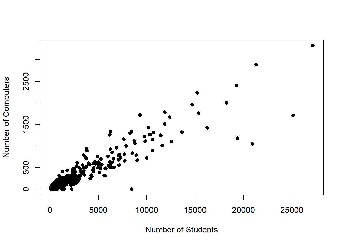
More students means more computers. In the regression we ran though all it knows is that schools with more computers do worse on math, but they can’t tell why. If larger schools have more computers AND do worse on tests, a bivariate regression can’t separate those effects on its own. We did bivariate regression in the last chapter, where we just look at two variables, one independent and one dependent (bivariate means two (bi) variables (variate)).

Multiple regression can help us try though. Multiple regression doesn’t mean running multiple regressions, it refers to including multiple variables in the same regression. Most of the tools we’ve learned so far only allow for two variables to be used, but with regression we can use many (many) more.

Let’s see what happens when we look at the relationship between the number of computers and math scores, controlling for the number of students at the school.

## 
## Call:
## lm(formula = math ~ computer + students, data = CASchools)
## 
## Residuals:
##    Min     1Q Median     3Q    Max 
## -48.89 -12.60  -1.03  12.49  52.10 
## 
## Coefficients:
##                Estimate  Std. Error t value   Pr(>|t|)    
## (Intercept) 654.1325380   1.0894390 600.431    < 2e-16 ***
## computer      0.0217002   0.0054817   3.959 0.00008860 ***
## students     -0.0028049   0.0006183  -4.537 0.00000748 ***
## ---
## Signif. codes:  0 '***' 0.001 '**' 0.01 '*' 0.05 '.' 0.1 ' ' 1
## 
## Residual standard error: 18.34 on 417 degrees of freedom
## Multiple R-squared:  0.04807,    Adjusted R-squared:  0.0435 
## F-statistic: 10.53 on 2 and 417 DF,  p-value: 0.00003461

This second regression shows something different. In the earlier regression, the number of computers was negative and not significant. Now? Now it’s positive and significant. So what happened?

We controlled for the number of students that are at the school, at the same time that we’re testing the relationship between computers and math scores. Don’t worry if that’s not clear yet, we’re going to spend some time on it. When I say “holding the number of students constant” it means comparing schools with different numbers of computers but that have the same number of students. If we compare two schools with the same number of students, we can then better identify the impact of computers.

We can interpret the variables in the same way as earlier when just testing one variable to some degree. We can see that a larger number of computers is associated with higher test scores, and that larger schools generally do worse on the math test.

Specifically, a one unit increase in computers is associated with an increase of math scores of.02 points, and that change is highly significant.

But our interpretation needs to add something more. With multiple regression what we’re doing is looking at the effect of each variable, while holding the other variable constant.

Specifically, a one unit increase in computers is associated with an increase of math scores of.002 points when holding the number of students constant, and that change is highly significant.

When we look at the effect of computers in this regression, we’re setting aside the impact of student enrollment and just looking at computers. And when we look at the coefficient for students, we’re setting aside the impact of computers and isolating the effect of larger school enrollments on test scores.

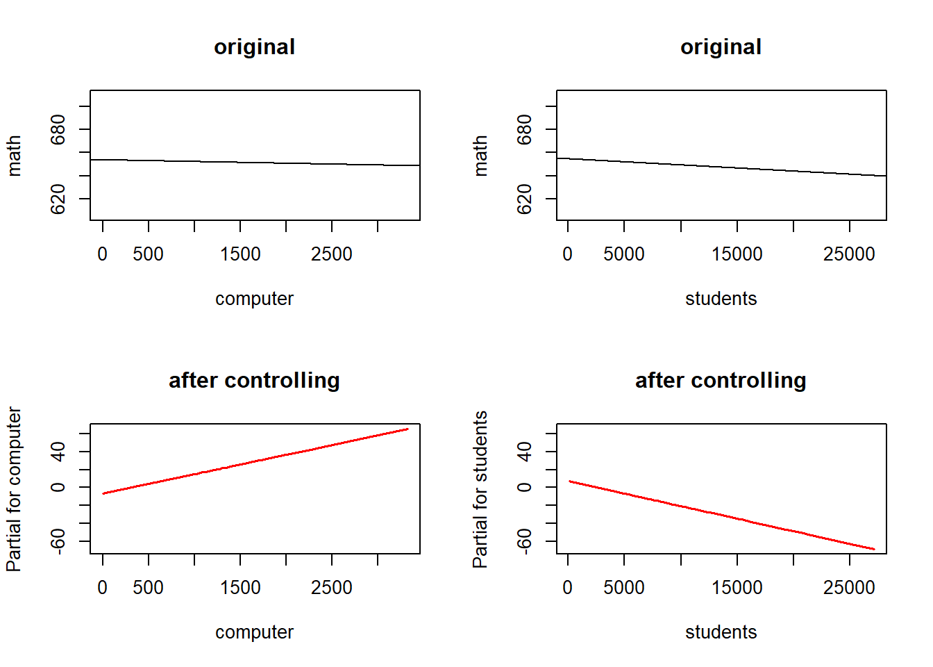
We looked at scatter plots and added a line to the graph to better understand the direction of relationships in the previous chapter. We can do that again, but it’s slightly different.

Here is the relationship of computers to math scores, and the relationship of computers to math scores holding students constant. That means we’re actually producing separate lines for both variables, but we’re doing that after accounting for the impact of computers on school enrollment, and school enrollment on computers.

We can also graph it in 3 dimensions, where we place the outcome on the z axis coming out of the paper/screen towards you.

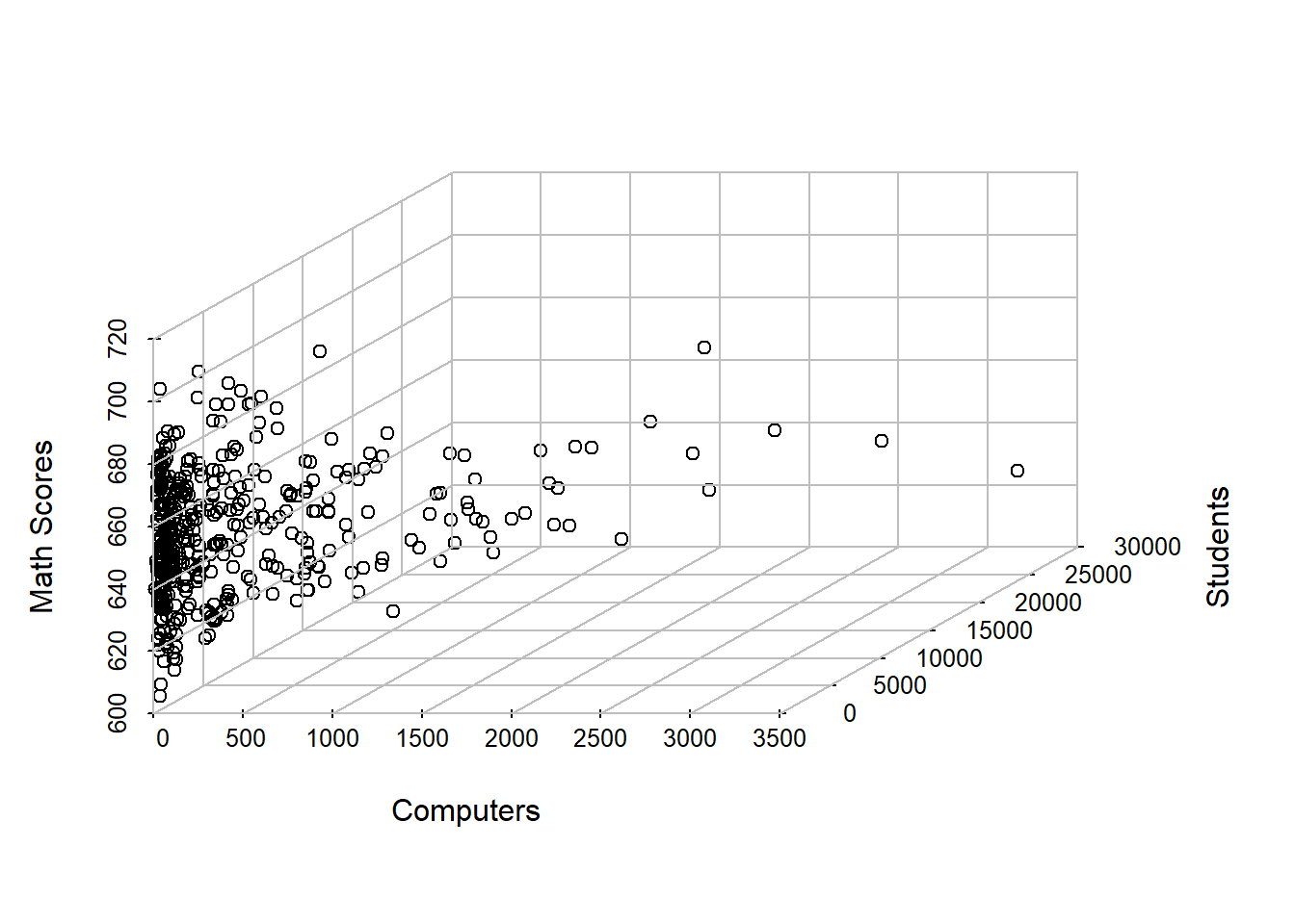
But I’ll be honest, that doesn’t really clarify it for me. Multiple regression is still about drawing lines, but it’s more of a theoretical line. It’s really hard to actually effectively draw lines as we move beyond two variables or two dimensions. Hopefully that logic of drawing a line and the equation of a line still makes sense for you, because it’s the same formula we use in interpreting multiple regressions.

What we’re figuring out with multiple regression is what part of math scores is determined uniquely by the student enrollment at a school and what part of math scores is determined uniquely by the number of computers. Once R figures that out it gives us the slope of two lines, one for computers and one for students. The line for computers slopes upwards, because the more computers a school has the better it’s students do, when we hold constant the number of students at the school. When we hold constant the number of computers, larger schools do worse on the math test.

I don’t expect that to fully make sense yet. Understanding what it means to “hold something constant” is pretty complex and theoretical, but it’s also important to fully utilizing the powers of regression. What this example illustrates though is the dangers inherent in using regression results, and the difficulty of using them to prove causality.

Let’s go back to the bivariate regression we did, just including the number of computers at a school and math test scores. Did that prove that computers don’t impact scores? No, even though that would be the correct interpretation of the results. But lets go back to what we need for causality…

Co-variation
Temporal Precedence
Elimination of Extraneous Variables or Hypotheses

We failed to eliminate extraneous variables. We tested the impact of computers, but we didn’t do anything to test any other hypotheses of what impacts math scores. We didn’t test whether other factors that impact scores (number of teachers, wealth of parents, size of the school) had a mediating relationship on the number of computers. Until we test every other explanation for the relationship, we haven’t really proven anything about computers and test scores. That’s why we need to take caution in doing regression. Yes, you can now do regression, and you can hopefully correctly interpret them. But correctly interpreting a regression, and doing a regression that proves something is a little more complicated. We’ll keep working towards that though.

15.1.1 Predicting Wages

To this point the book has attempted to avoid touching on anything that is too controversial. Statistics is a math, so it’s a fairly apolitical field, but it can be used to support political or controversial matters. We’re going to wade into one in this chapter, to try and show the way that statistics can let us get at some of the thorny issues our world deals with. In addition, this example should help to clarify what it means to “hold something constant”.

We’ll work with the same income data we used in the last chapter from the Panel Study of Income Dynamics from 1982. Just to remind you, these are the variables we have available.

experience - Years of full-time work experience.
weeks - Weeks worked.
occupation - factor. Is the individual a white-collar (“white”) or blue-collar (“blue”) worker?
industry - factor. Does the individual work in a manufacturing industry?
south - factor. Does the individual reside in the South?
smsa - factor. Does the individual reside in a SMSA (standard metropolitan statistical area)?
married - factor. Is the individual married?
gender - factor indicating gender.
union - factor. Is the individual’s wage set by a union contract?
education - Years of education.
ethnicity - factor indicating ethnicity. Is the individual African American (“afam”) or not (“other”)?
wage - Wage.

Let’s say we wanted to understand wage discrimination on the basis of race or ethnicity Do African Americans earn less than others in the workplace? Let’s see what this data tells us.

And a note before we begin. The variable ethnicity has two categories, “afam” which indicates African American or “other” which means anything but African American. Obviously, that captures a lot modernly, but in the 1980 that generally can be understood to generally be white people. I’ll generally just refer to it as other races in the text though.

ethnicity	wage
other	1174
afam	808.5

The average wage for African Americans in the data is 808.5, and for others the average wage is 1174. That means that African Americans earn (in this really specific data set) 61% of how much men earn 365.5 less.

Let’s say we take that fact to someone that doesn’t believe that African Americans are discriminated against. We’ll call them you’re “contrarian friend”, you can fill in other ideas of what you’d think about that person. What will their response be? Probably that it isn’t evidence of discrimination, because of course African Americans earn less, they’re less likely to work in white collar jobs. And people that work in white collar jobs earn more, so that’s the reason African Americans earn less. It’s not discrimination, it’s just that they work different jobs.

And on the surface, they’d be right. African Americans are more likely to work in blue collar jobs (65% to 50%), and blue collar jobs earn less (956 for blue collar jobs to 1350 for white collar jobs).

ethnicity	blue_collar
other	0.5018
afam	0.6512

blue_collar	wage
0	1350
1	956.4

So what we’d want to do then is compare African Americans to others that both work blue collar jobs, and African Americans to others working white collar jobs. If there is a difference in wages between two people working the same job, that’s better evidence that the pay gap is a result not of their occupational choices but their race.

We can visualize that with a two by two chart.

##           ethnicity
## occupation     other     afam
##      white 1373.1527 918.4667
##      blue   977.2635 749.5357

Let’s work across that chart to see what it tells us. A 2 by 2 chart like that is called a cross tab because it let’s us tabulate figures across different characteristics of our data. They can be a methodologically simple way (we’re just showing means/averages there) to tell a story if the data is clear.

So what do we learn? Looking at the top row, white collar workers that are labeled other for ethnicity earn on average $1373. And white collar workers that are African American earn $918. Which means that for white collar workers, African Americans earn $455 less. For blue collar workers, other races earn $977, while African Americans earn $749. That’s a gap of $228. So the size of the gap is different depending on what a persons job is, but African American’s earn less regardless of their job. So it isn’t just that African Americans are less likely to work white collar jobs that drives their lower wages. Even those in white collar jobs earn less. In fact, African Americans in white collar jobs earn less on average than other races working blue collar jobs!

This is what it means to hold something constant. In that table above we’re holding occupation constant, and comparing people based on their race to people of another race that work the same job. So differences in those jobs aren’t influencing our results now, we’ve set that effect aside for the moment.

And we can do that automatically with regression, like we did when we looked at the effect of computers on math scores, while holding the impact of school enrollment constant.

## 
## Call:
## lm(formula = wage ~ ethnicity + occupation, data = PSID1982)
## 
## Residuals:
##     Min      1Q  Median      3Q     Max 
## -1018.6  -325.2   -40.6   215.3  3734.4 
## 
## Coefficients:
##                Estimate Std. Error t value  Pr(>|t|)    
## (Intercept)     1365.62      28.91  47.234   < 2e-16 ***
## ethnicityafam   -309.14      77.43  -3.992 0.0000737 ***
## occupationblue  -380.89      40.11  -9.495   < 2e-16 ***
## ---
## Signif. codes:  0 '***' 0.001 '**' 0.01 '*' 0.05 '.' 0.1 ' ' 1
## 
## Residual standard error: 487.6 on 592 degrees of freedom
## Multiple R-squared:  0.1599, Adjusted R-squared:  0.157 
## F-statistic: 56.32 on 2 and 592 DF,  p-value: < 2.2e-16

Based on that regression results, African Americans earn $309 less than other races when holding occupation constant, and that effect is highly significant. And blue collar workers earn $380 less than white collar workers when holding race constant, and that effect is significant too.

So have we proven discrimination in wages? Probably not yet for the contrarian friend. Without pause they’ll likely say that education is also important for wages, and African Americans are less likely to go to college. And in the data they’d be correct. On average African Americans completed 11.65 years of education, and other races completed 12.94.

ethnicity	education
other	12.94
afam	11.65

So let’s add that to our regression too.

## 
## Call:
## lm(formula = wage ~ ethnicity + occupation + education, data = PSID1982)
## 
## Residuals:
##     Min      1Q  Median      3Q     Max 
## -1050.9  -310.9   -46.1   218.6  3591.1 
## 
## Coefficients:
##                Estimate Std. Error t value Pr(>|t|)    
## (Intercept)     441.407    135.830   3.250 0.001221 ** 
## ethnicityafam  -261.577     74.826  -3.496 0.000508 ***
## occupationblue -158.141     50.166  -3.152 0.001702 ** 
## education        62.793      9.033   6.952 9.59e-12 ***
## ---
## Signif. codes:  0 '***' 0.001 '**' 0.01 '*' 0.05 '.' 0.1 ' ' 1
## 
## Residual standard error: 469.2 on 591 degrees of freedom
## Multiple R-squared:  0.2234, Adjusted R-squared:  0.2194 
## F-statistic: 56.66 on 3 and 591 DF,  p-value: < 2.2e-16

Now with the ethnicity variable we’re comparing people of different ethnicities that have the same occupation and education. And what do we find? Even holding both of those constant, we would expect an African American worker to earn $262 less, and that is highly significant.

What your contrarian friend is doing is proposing alternative variables and hypotheses that explain the gap in earnings for African Americans. And while those other things do make a difference they don’t explain fully why African Americans earn less than others. We have shrunk the gap somewhat. Originally the gap was 465, which fell to 309 when we held occupation constant and now 262 with the inclusion of education. So those alternative explanations do explain a portion of why African Americans earned less, it was because they had lower-status jobs and less education (setting aside the fact that their lower-status jobs and less education may be the result of discrimination).

So what else do we want to include to try and explain that difference in wages? We can insert all of the variables in the data set to see if there is still a gap in wages between African Americans and others.

## 
## Call:
## lm(formula = wage ~ ethnicity + occupation + education + experience + 
##     weeks + industry + south + smsa + married + gender + union, 
##     data = PSID1982)
## 
## Residuals:
##     Min      1Q  Median      3Q     Max 
## -1008.8  -279.8   -37.4   196.7  3482.1 
## 
## Coefficients:
##                Estimate Std. Error t value Pr(>|t|)    
## (Intercept)     -39.735    234.478  -0.169 0.865491    
## ethnicityafam  -167.249     71.815  -2.329 0.020207 *  
## occupationblue -180.637     48.699  -3.709 0.000228 ***
## education        65.257      8.698   7.503 2.34e-13 ***
## experience        6.578      1.744   3.772 0.000179 ***
## weeks             2.962      3.529   0.839 0.401726    
## industryyes      86.693     38.443   2.255 0.024496 *  
## southyes        -59.662     40.791  -1.463 0.144110    
## smsayes         169.833     38.978   4.357 1.56e-05 ***
## marriedyes       85.620     64.500   1.327 0.184883    
## genderfemale   -344.516     80.124  -4.300 2.00e-05 ***
## unionyes         25.782     41.761   0.617 0.537225    
## ---
## Signif. codes:  0 '***' 0.001 '**' 0.01 '*' 0.05 '.' 0.1 ' ' 1
## 
## Residual standard error: 429.7 on 583 degrees of freedom
## Multiple R-squared:  0.3575, Adjusted R-squared:  0.3454 
## F-statistic: 29.49 on 11 and 583 DF,  p-value: < 2.2e-16

Controlling for occupation, education, experience, weeks worked, the industry, the region of employment, whether they are married, their gender, and their union status, does ethnicity make a difference in earnings? Yes, if you found two workers that had the same values for all of those variables except that they were of different races, the African American would still likely earn less.

In our regression African Americans earn $167 less when holding occupation, education, experience, weeks worked, the industry, region, marriage, gender, and their union status constant, and that effect is still statistically significant.

The contrarian friend may still have another alternative hypothesis to attempt to explain away that result, but unfortunately that’s all the data will let us test.

What we’re attempting to do is minimize what is called the missing variable bias. If there is a plausible story that explains our result, whether one is predicting math test scores or wages or whatever else, if we fail to account for that explanation our model may be misleading. It was misleading to say that computers don’t increase math test scores when we didn’t control for the effect of larger school sizes.

What missing variables do we not have that may explain the difference in earnings between African Americans and others? We don’t know who is a manager at work or anything about job performance, and both of those should help explain why people earn more. So we haven’t removed our missing variable bias, the evidence we can provide is limited by that. But based on the evidence we can generate, we find evidence of racial discrimination in wages.

And I should again emphasize, even if something else did explain the gap in earnings between African Americans and others it wouldn’t prove there wasn’t discrimination in society. If differences in occupation did explain the racial gap in wages, that wouldn’t prove the discrimination didn’t push African Americans towards lower paying jobs.

But the work we’ve done above is similar to what a law firm would do if bringing a lawsuit against a large employer for wage discrimination. It’s hard to prove discrimination in individual cases. The employer will always just argue that John is a bad employee, and that’s why they earn less than their coworkers. Wage discrimination suits are typically brought as class action suits, where a large group of employees sues based on evidence that even when accounting for differences in specific job, and job performance, and experience, and other things there is still a gap in wages.

I should add a note about interpretation here. It’s the researcher that has to identify what they different coefficients means in the real world. We can talk about discrimination because of differences in earnings for African Americans and others, but we wouldn’t say that blue collar workers are discriminated against because they earn less than white collar workers. It’s unlikely that someone would say that people with more experience earning more is the result of discrimination. These are interpretations that we layer on to the analysis based on our expectations and understanding of the research question.

15.1.2 Predicting Affairs

Regression can be used to make predictions and learn more about the world in all sorts of contexts. Let’s work through another example, with a little more focus on the interpretation.

We’ll use a data set called Affairs, which unsurprisingly has data about affairs. Or more specifically, about people, and whether or not they have had an affair.

In the data set there are 10 variables.

affairsany - coded as 0 for those who haven’t had an affair and 1 for those who have had any number of affairs. This will be the dependent variable.
gender - either male or female
age - respondents age
yearsmarried - number of years of current marriage
children - are there children from the marriage
religiousness - scaled from 1-5, with 1 being anti religion and 5 being very religious
education -years of education
occupation - 1-7 based on a specific system of rating for occupations
rating 1-5 based on how happy the respondent reported their marriage being.

So we can throw all of those variables into a regression and see which ones have the largest impact on the likelihood someone had an affair. But before that we should pause to make predictions. We shouldn’t just include a variable just for laughs - we should have a reason for including it. We should be able to make a prediction for whether it should increase or decrease the dependent variable.

So what effect do you think these independent variables will have on the chances of someone having had an affair?

gender - I would guess their (on average) higher libidos and lower levels of concern about childbearing will lead to more affairs.
age - Young people are typically a little less ready for long term commitments, and a bit more irrational and willing to take chances, so age should decrease affairs. Although being older does give you more time to of had an affair. *yearsmarried - Longer marriages should be less likely to contain an affair. If someone was going to have an affair, i would expect it to happen earlier, and such things often end marriages.
children - Children, and avoiding hurting them, are hopefully a good reason for people to avoid having affairs.
religiousness - most religions teach that affairs are wrong, so I would guess people that are more religious are less likely to have affairs
education and occupation - I actually can’t make a prediction for what effect education or occupation have on affairs, and since I don’t think they’ll impact the dependent variable I wouldn’t include them in the analysis if I was doing this for myself. But I’ll keep them here as an example to talk about later.
rating - happier marriages will likely produce fewer affairs, in large part because it’s often unhappiness that makes couples stray.

Those arguments may be wrong or right. And they certainly wont be right in every case in the data - there will be counter examples. What I’ve tried to do is lay out predictions, or hypotheses, for what I expect the model to show us. Let’s test them all and see what predicts whether someone had an affair.

## 
## Call:
## lm(formula = affairsany ~ gender + age + yearsmarried + children + 
##     religiousness + education + occupation + rating, data = Affairs)
## 
## Residuals:
##     Min      1Q  Median      3Q     Max 
## -0.6336 -0.2691 -0.1632  0.1151  1.0659 
## 
## Coefficients:
##                Estimate Std. Error t value     Pr(>|t|)    
## (Intercept)    0.736107   0.151502   4.859 0.0000015148 ***
## gendermale     0.045201   0.040022   1.129     0.259180    
## age           -0.007420   0.003013  -2.463     0.014057 *  
## yearsmarried   0.015981   0.005491   2.911     0.003743 ** 
## childrenyes    0.054487   0.046642   1.168     0.243198    
## religiousness -0.053698   0.014881  -3.608     0.000334 ***
## education      0.003078   0.008542   0.360     0.718699    
## occupation     0.005913   0.011838   0.499     0.617643    
## rating        -0.087455   0.015984  -5.472 0.0000000659 ***
## ---
## Signif. codes:  0 '***' 0.001 '**' 0.01 '*' 0.05 '.' 0.1 ' ' 1
## 
## Residual standard error: 0.4122 on 592 degrees of freedom
## Multiple R-squared:  0.1066, Adjusted R-squared:  0.09452 
## F-statistic: 8.829 on 8 and 592 DF,  p-value: 1.884e-11

What do you see as the strongest predictors of whether someone had an affair? Let’s start by identifying what was highly statistically significant. Religiousness and rating both had p-values below .001, so we can be very confident that in the population people who are more religious and who report having happier marriages are both less likely to have affairs. Let’s interpret that more formally.

For each one unit increase in religiousness an individual’s chances of having an affair decrease by .05 holding their gender, age, years married, children, education, occupation and rating constant, and that change is significant.

That’s a long list of things we’re holding constant! When you get past 2 or 3 control variables, or when you’re describing different variables from the same model you can use “holding all else constant” in place of the list.

For each one unit increase in the happiness rating of a marriage an individual’s chances of having an affair decrease by .09, holding all else constant, and that change is significant.

What else that we included in the model is useful for predicting whether someone had an affair?

Age and years married both reach statistical significance. As individuals get older, their chances of having an affair decrease, as I predicted.

However, as their marriages get longer the chances of having had an affair increase, not decrease as I thought Interesting! Does that mean I should go back and change my prediction? No. What it likely means is that some of my assumptions were wrong, so I should update them and discuss why I was wrong (in the conclusion if this was a paper). If we only used regression to find things that we already know, we wouldn’t learn anything new. It’s still good that I made a prediction though because that highlights that the result is a little weird (to my eyes) or may be more surprising to the readers. Imagine if you found that a new jobs program actually lowered participants incomes, that would be a really important outcome of your research and just as valuable as if you’d found that incomes increase.

A surprising finding could also be evidence that there’s something wrong in the data. Did we enter years of marriage correctly, or did we possibly reverse it where longer marriages are actually coded as lower numbers. That’d be odd in this case, but it’s always worth thinking that possibility through. If I got data that showed college graduates earned less than those without a high school degree I’d be very skeptical of the data, because that would go against everything we know. It might just be an odd, fluky one-time finding, or it could be evidence something is wrong in the data.

Okay, what about everything else? All the other variables are insignificant. Should we remove them from the analysis, since they don’t have a significant effect on our dependent variable? It depends. Insignificant variables can be worth including in most cases in order to show that they don’t have an effect on the outcome. It’s worth knowing that gender and children don’t have an effect on affairs in the population. We had a reason to think they would, and it turns out they don’t really have much of an influence on whether someone has sex outside their marriage. That’s good to know.

I didn’t have a prediction for education or occupation though, and the fact they are insignificant means they aren’t really worth including. I’m not testing any interesting ideas about what affects affairs with those variables, they’re just being included because they’re in the data. That’s not a good reason for them to be there, we want to be testing something with each variable we include.

15.2 Practice

In truth, we haven’t done a lot of new work on code in this chapter. We’ve more so focused on this big idea of what it means to go from bivariate regression to multivariate regression. So we wont do a lot of practice, because the basic structure we learned in the last chapter drives most of what we’ll do.

We’ll read in some new data, that’s on Massachusetts schools and test scores there. It’s similar to the California Schools data, but from Massachusetts for variety.

##   X district municipality expreg expspecial expbil expocc exptot scratio
## 1 1        1     Abington   4201    7375.69      0      0   4646    16.6
## 2 2        2        Acton   4129    8573.99      0      0   4930     5.7
## 3 3        3     Acushnet   3627    8081.72      0      0   4281     7.5
## 4 4        5       Agawam   4015    8181.37      0      0   4826     8.6
## 5 5        7     Amesbury   4273    7037.22      0      0   4824     6.1
## 6 6        8      Amherst   5183   10595.80   6235      0   6454     7.7
##   special lunch stratio income score4 score8  salary   english
## 1    14.6  11.8    19.0 16.379    714    691 34.3600 0.0000000
## 2    17.4   2.5    22.6 25.792    731     NA 38.0630 1.2461059
## 3    12.1  14.1    19.3 14.040    704    693 32.4910 0.0000000
## 4    21.1  12.1    17.9 16.111    704    691 33.1060 0.3225806
## 5    16.8  17.4    17.5 15.423    701    699 34.4365 0.0000000
## 6    17.2  26.8    15.7 11.144    714     NA      NA 3.9215686

We’ll focus on 4 of those variable, and try to figure out what predicts how schools do on tests in 8th grade (score8).

score8 - test scores for 8th graders
exptot - total spending for the school
english - percentage of students that don’t speak english as their native language
income - income of parents

Let’s start by practicing writing a regression to look at the impact of spending (exptot) on test scores.

## 
## Call:
## lm(formula = score8 ~ exptot, data = MASchools)
## 
## Residuals:
##     Min      1Q  Median      3Q     Max 
## -62.178 -11.611   0.756  14.735  46.702 
## 
## Coefficients:
##               Estimate Std. Error t value Pr(>|t|)    
## (Intercept) 675.361287   8.938904  75.553  < 2e-16 ***
## exptot        0.004218   0.001611   2.618  0.00961 ** 
## ---
## Signif. codes:  0 '***' 0.001 '**' 0.01 '*' 0.05 '.' 0.1 ' ' 1
## 
## Residual standard error: 20.72 on 178 degrees of freedom
##   (40 observations deleted due to missingness)
## Multiple R-squared:  0.03708,    Adjusted R-squared:  0.03167 
## F-statistic: 6.854 on 1 and 178 DF,  p-value: 0.009608

That should look very similar to the last chapter. And we can interpret it the same way.

For each one unit increase in spending, we observe a .004 increase in test scores for 8th graders, and that change is significant.

Let’s add one more variable to the regression, and now include english along with exptot. To include an additional variable we just place a + sign between the two variables, as shown below.

## 
## Call:
## lm(formula = score8 ~ exptot + english, data = MASchools)
## 
## Residuals:
##     Min      1Q  Median      3Q     Max 
## -37.343 -11.921  -0.496  11.467  40.196 
## 
## Coefficients:
##               Estimate Std. Error t value    Pr(>|t|)    
## (Intercept) 664.615475   7.254776  91.611     < 2e-16 ***
## exptot        0.007136   0.001326   5.382 0.000000231 ***
## english      -4.134282   0.414805  -9.967     < 2e-16 ***
## ---
## Signif. codes:  0 '***' 0.001 '**' 0.01 '*' 0.05 '.' 0.1 ' ' 1
## 
## Residual standard error: 16.63 on 177 degrees of freedom
##   (40 observations deleted due to missingness)
## Multiple R-squared:  0.3832, Adjusted R-squared:  0.3763 
## F-statistic: 54.99 on 2 and 177 DF,  p-value: < 2.2e-16

Each one unit increase in spending is associated with a .007 increase in test scores for 8th graders, holding the percentage of english speakers constant, and that change is significant.

Each one unit increase in the percentage of students that don’t speak english as natives is associated with a 4.1 decrease in test scores for 8th graders, holding the spending constant, and that change is significant.

And one more, let’s add one more variable: income.

## 
## Call:
## lm(formula = score8 ~ exptot + english + income, data = MASchools)
## 
## Residuals:
##     Min      1Q  Median      3Q     Max 
## -29.742  -6.920  -0.678   6.037  41.988 
## 
## Coefficients:
##               Estimate Std. Error t value Pr(>|t|)    
## (Intercept) 659.891542   4.837735 136.405  < 2e-16 ***
## exptot       -0.001878   0.001068  -1.758   0.0805 .  
## english      -2.246437   0.303501  -7.402 5.32e-12 ***
## income        2.754197   0.184124  14.958  < 2e-16 ***
## ---
## Signif. codes:  0 '***' 0.001 '**' 0.01 '*' 0.05 '.' 0.1 ' ' 1
## 
## Residual standard error: 11.06 on 176 degrees of freedom
##   (40 observations deleted due to missingness)
## Multiple R-squared:  0.7285, Adjusted R-squared:  0.7238 
## F-statistic: 157.4 on 3 and 176 DF,  p-value: < 2.2e-16

Interesting, spending actually lost its significance in that final regression and change directions.

Each one unit increase in spending is associated with a .002 decrease in test scores for 8th graders when holding the percentage of english speakers and parental income constant, but that change is insignificant.

Each one unit increase in the percentage of students that don’t speak english as natives is associated with a 2.2 decrease in test scores for 8th graders when holding spending and parental income constant, and that change is significant.

Each one unit increase in parental income is associated with a 2.8 increase in test scores for 8th graders when holding spending and the percentage of english speakers constant, and that change is significant.

The following video demonstrates the coding steps done above.