20 Spatial Models
“everything is related to everything else, but near things are more related than distant things.” -The First Law of Geography, Waldo Tobler (1970)
20.1 Concepts
Spatial data allows us to test for and correct one potential issue that can be present in our models. As was discussed in an earlier chapter, the observations of our data must be independent. However, whenever we use spatial data that assumption may be violated. In that chapter I described temporal autocorrelation, where observations of an individual were unlikely to change significantly over time. Observations can also be spatially autocorrelated
Take for instance a demographic characteristic such as median income. If I look at median income for the country at the county level, do you think they will be randomly distributed? Let’s look below.
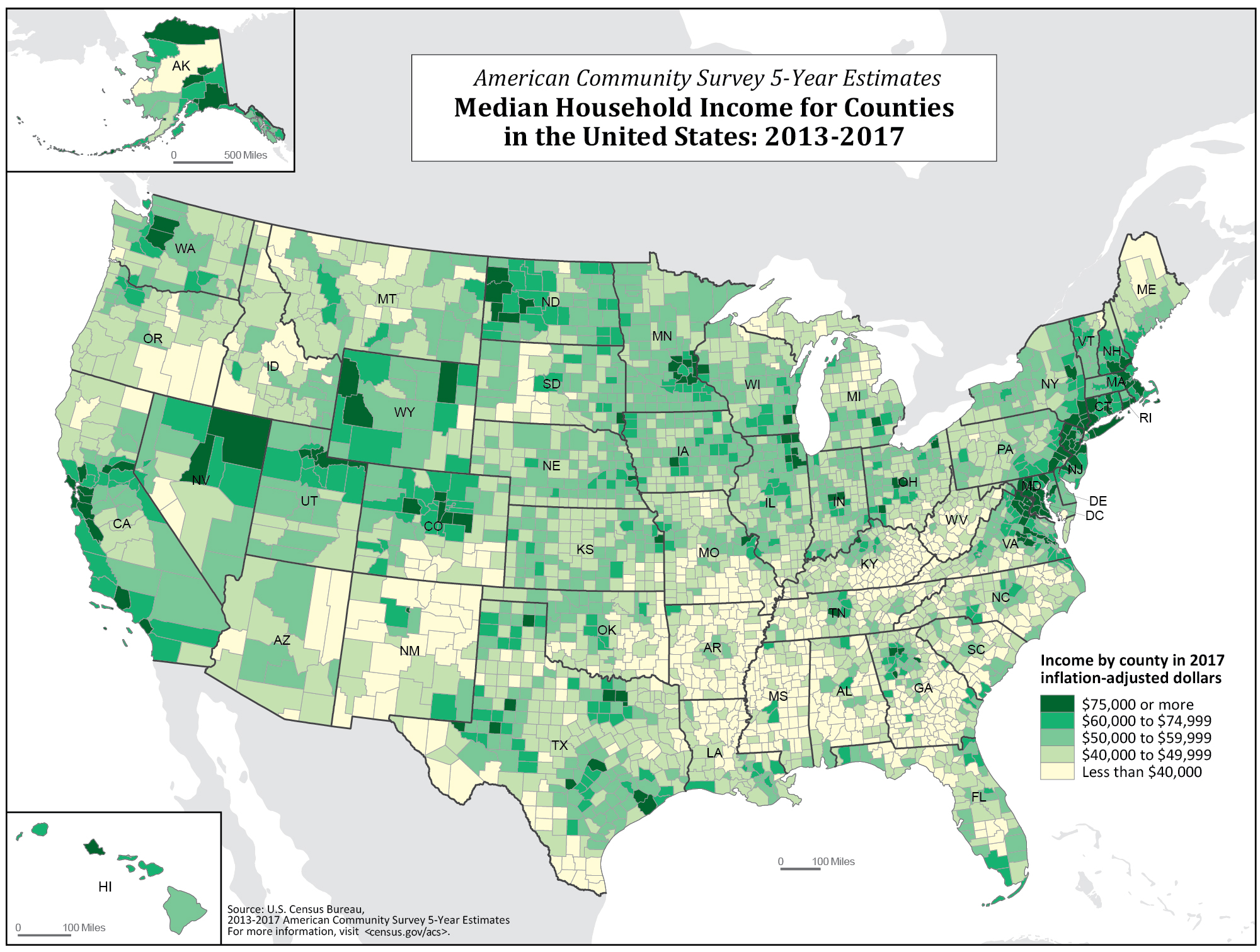
It appears that rather than being randomly distributed, median incomes are spatially connected. Richer counties tend to be closer to richer counties, and poorer counties tend to be nearer to poorer counties. In part that’s because of spillovers and regional resources - a county near a valuable natural resource like a port is going to benefit multiple counties. And richer counties can create additional commerce with nearby counties (shopping, travel, etc.) which creates widespread benefits. The opposite trends occur in poorer counties.
That is an example of spatial dependence. Rather than each county being independent, knowing the median income of nearby counties can help you to predict the median income of another county. Conversely, with a simple random sample, knowing whether row 8 voted does not help you predict anything about row 9.
This chapter will walk you through testing for spatial dependences, and techniques for correcting for those issues.
20.1.1 Spatial autocorrelation
Spatial autocorrelation refers to how strongly objects correlate with other nearby objects across a spatial area. Generally, we think of correlation as being internal to an observation, in the way that height and weight correlate. Here we’re concerned with the correlation between different objects, such as neighborhoods, counties, cities, or states. When nearby objects tend to be higher or lower on a given value (like median income) we refer to that as spatial autocorrealtion.
Let’s jump into an example. In the summer of 2020 I wrote a paper with some colleagues looking at what neighborhoods (census tracts) in Louisiana had the largest outbreaks of COVID through May of that year. We’ll use that data below and explore the potential issues of spatial autocorrelation that were present.
## OGR data source with driver: ESRI Shapefile
## Source: "C:\Users\evanholm\Dropbox\Papers\Finished\Neighborhood COVID\Data\tl_2019_22_tract\tl_2019_22_tract.shp", layer: "tl_2019_22_tract"
## with 1148 features
## It has 12 fields
## Integer64 fields read as strings:  ALAND AWATER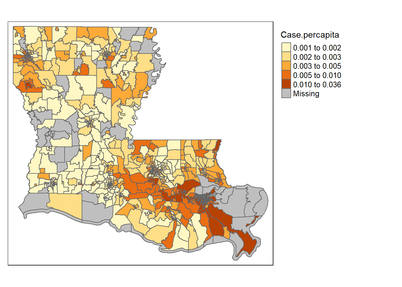
First, you’ll want to run a basic OLS regression in order to identify whether there are any problems in your data. The dependent variable for the model was the log of the number of Covid-19 cases per 1000 residents in each county. In these models we controlled for a bunch of community demographics: the population density, the percentage of residents that take public transit to work, the % of residents that work in a different county, the # of employment in tourism industries, % college graduates, % in poverty, % without health insurance, % Black, % Latinx, % Asian, % Other Minority, a diversity index, the % over the age of 70, and % Male.
So we start with an OLS regression.
##
## Call:
## lm(formula = cpcln ~ log(popdens) + pubtransit + outsidecounty +
##     tourismemp + collegepct + povpct + noinsurance + blackpct +
##     hisppct + asianpct + otherracepct + DiversityIndex + over70pct +
##     male, data = tractLA2@data)
##
## Residuals:
##      Min       1Q   Median       3Q      Max
## -1.47786 -0.36455 -0.00906  0.32609  1.80388
##
## Coefficients:
##                Estimate Std. Error t value Pr(>|t|)
## (Intercept)    -0.39284    0.23111  -1.700  0.08946 .
## log(popdens)    0.10088    0.01233   8.179 8.19e-16 ***
## pubtransit      4.06333    0.46030   8.828  < 2e-16 ***
## outsidecounty   1.32509    0.10045  13.191  < 2e-16 ***
## tourismemp      0.53975    0.31477   1.715  0.08669 .
## collegepct      0.17274    0.13784   1.253  0.21043
## povpct         -1.09587    0.19405  -5.647 2.10e-08 ***
## noinsurance    -0.97622    0.41245  -2.367  0.01812 *
## blackpct        1.41707    0.09042  15.672  < 2e-16 ***
## hisppct         3.33953    0.36655   9.111  < 2e-16 ***
## asianpct        2.20238    0.52071   4.230 2.55e-05 ***
## otherracepct    2.02512    0.69106   2.930  0.00346 **
## DiversityIndex -0.22833    0.11828  -1.930  0.05382 .
## over70pct       3.29006    0.43666   7.535 1.06e-13 ***
## male            0.24399    0.37692   0.647  0.51756
## ---
## Signif. codes:  0 '***' 0.001 '**' 0.01 '*' 0.05 '.' 0.1 ' ' 1
##
## Residual standard error: 0.5144 on 1048 degrees of freedom
##   (85 observations deleted due to missingness)
## Multiple R-squared:  0.5444, Adjusted R-squared:  0.5383
## F-statistic: 89.45 on 14 and 1048 DF,  p-value: < 2.2e-16
On it’s surface, that model looks pretty good. There were lots of significant variables, and the adjusted R-squared is fairly high. But as we know, that doesn’t help us assess whether any violations are present in the OLS.
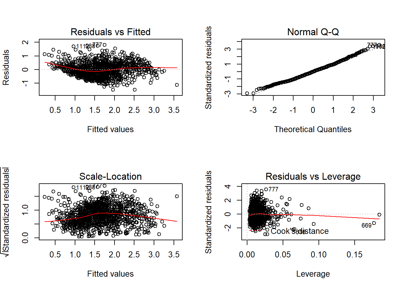
Those look okay. The Residuals vs. Fitted shows that the residuals are a bit squeezed at the beginning and end, which can be concerning. But the Normal Q-Q Plot looks great, and there aren’t any outliers to be worried about.
So let’s look closer at the residuals. What we’re concerned with is whether our data is spatially correlated, and as a result whether our residuals are spatially correlated. If our dependent variable has clusters, it’ll be likely that our model will underpredict certain areas, and overpredict others. As a result, the residuals won’t be randomly distributed across the state. One way to see if that is the case is to map the residuals.
##
## Call:
## lm(formula = cpcln ~ log(popdens) + pubtransit + outsidecounty +
##     tourismemp + collegepct + povpct + noinsurance + blackpct +
##     hisppct + asianpct + otherracepct + DiversityIndex + over70pct +
##     male, data = covid.cnty2)
##
## Residuals:
##     Min      1Q  Median      3Q     Max
## -1.5030 -0.3766 -0.0068  0.3087  1.9041
##
## Coefficients:
##                Estimate Std. Error t value Pr(>|t|)
## (Intercept)    -0.39405    0.27318  -1.442  0.14952
## log(popdens)    0.10303    0.01346   7.654 5.17e-14 ***
## pubtransit      4.26734    0.76369   5.588 3.08e-08 ***
## outsidecounty   1.25027    0.10799  11.578  < 2e-16 ***
## tourismemp      0.50733    0.37787   1.343  0.17975
## collegepct     -0.07771    0.16337  -0.476  0.63445
## povpct         -1.17530    0.21985  -5.346 1.15e-07 ***
## noinsurance    -1.15469    0.47328  -2.440  0.01490 *
## blackpct        1.39616    0.10135  13.776  < 2e-16 ***
## hisppct         3.53221    0.40809   8.655  < 2e-16 ***
## asianpct        1.73022    0.59077   2.929  0.00349 **
## otherracepct    1.73110    0.73408   2.358  0.01858 *
## DiversityIndex -0.22379    0.13220  -1.693  0.09084 .
## over70pct       3.37763    0.50341   6.709 3.52e-11 ***
## male            0.39023    0.44405   0.879  0.37976
## ---
## Signif. codes:  0 '***' 0.001 '**' 0.01 '*' 0.05 '.' 0.1 ' ' 1
##
## Residual standard error: 0.5138 on 869 degrees of freedom
## Multiple R-squared:  0.5007, Adjusted R-squared:  0.4926
## F-statistic: 62.23 on 14 and 869 DF,  p-value: < 2.2e-16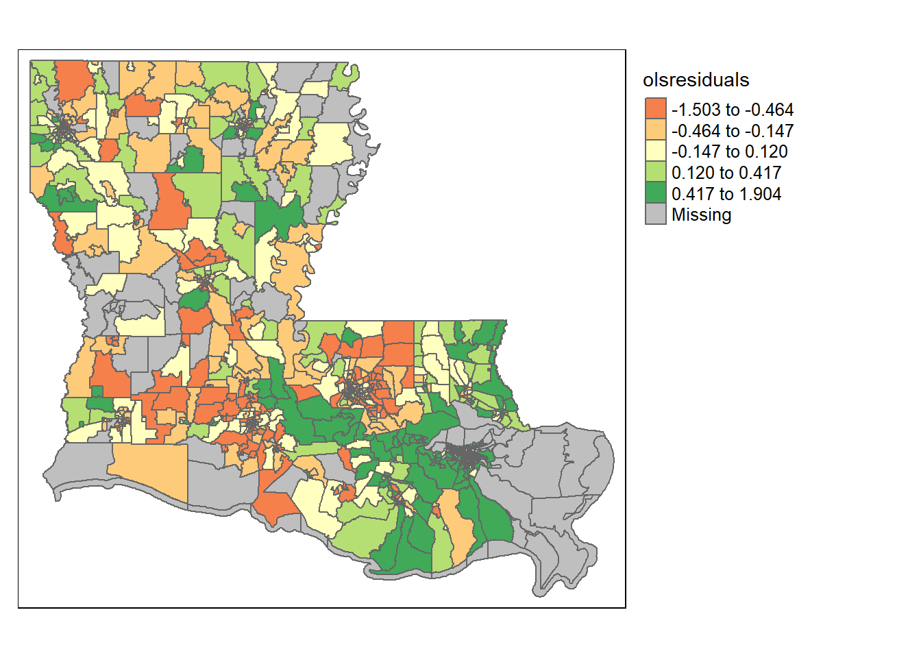
Do the residuals look randomly distributed there? Not really. High residuals are often near other high residuals, and low residuals are near other low residuals. That’s bad. It means our errors are correlated and our observations aren’t independent.
We can also look for clustering using what’s called a Moran’s I test. Moran’s I tests for whether or not your residuals are clustered more than chance would predict; a significant p-value indicates that yes, the data is clustered.
FALSE
FALSE   Global Moran I for regression residuals
FALSE
FALSE data:
FALSE model: lm(formula = cpcln ~ log(popdens) + pubtransit +
FALSE outsidecounty + tourismemp + collegepct + povpct + noinsurance +
FALSE blackpct + hisppct + asianpct + otherracepct + DiversityIndex +
FALSE over70pct + male, data = covid.cnty2)
FALSE weights: rwm
FALSE
FALSE Moran I statistic standard deviate = 5.1441, p-value =
FALSE 0.0000002689
FALSE alternative hypothesis: two.sided
FALSE sample estimates:
FALSE Observed Moran I      Expectation         Variance
FALSE     0.1120621369    -0.0025595422     0.0004965039
The p-value is well below the .05 cutoff, which indicates that our residuals are clustered, which aligns with what we saw visually.
Now that we know there is a problem, let’s work through two solutions: a spatial error model and a spatially lagged model. They attempt to correct for that issue slightly differently.
20.1.2 Neighbors
In order to address the spatial correlation for our residuals with either model we’ll need to tell R how each unit is clustered. Essentially, if we think there are issues between nearby units, we need to first identify which units are near other units. We can do that by creating a queens neighbors matrix, which might sound fancier than it is.
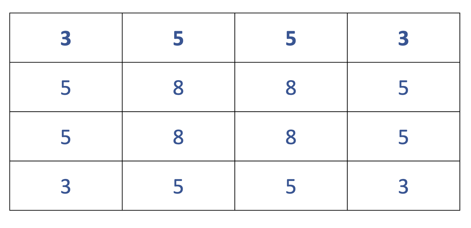
You calculate a queen’s neighbors by counting all polygons that border on each polygon. It’s called a queen’s neighbors because it can move in all directions. There are other systems, such as a rook’s neighbors where diagonal neighbors aren’t counted or a bishops neighbor’s where you onyl count the diagonal neighbors, but queen’s are the most common and are the default for the calculation we do below. The image below counts the number of neighbors for each block. With queen’s neighbors, any parts touching constitutes a neighbor.
## Neighbour list object:
## Number of regions: 1148
## Number of nonzero links: 7024
## Percentage nonzero weights: 0.5329675
## Average number of links: 6.118467
20.1.3 Spatial Models
With that in place, we can begin our modeling. We have two types of spatial models that we will describe. Essentially, they disagree about how significant of a problem the spatial autocorrelation of our residuals is. A spatial error model treats it as something of a nuisance, and handles it as if the spatial clustering was an accident. On the other hand, a spatial lag model takes that issue more seriously, and models the process as if there is spatial autocorrelation is evidence that there ais something different about the areas that are causing the clustering.
Let me try to illustrate that. Have you ever noticed that auto dealerships tend to be near other auto dealerships? Do you think that’s an accident or not? That’s one of the things we’re trying to determine in choosing a spatial lag or spatial error model. If we think it’s an accident, and auto dealers each independently choose where to locate and ended up near each other, then a spatial error model should be better. If there’s an underlying reason they’re clustered (and other areas don’t have auto dealers) then the spatial lag should do better. Luckily, we don’t really have to rely on theory, as it’s often the case that spatial clustering is the result of both accident and spillovers between different phenomena. Rather, there are well established statistical tests that can help us decide which model we want to utilize.
So I’ll first run the spatial error model below. The output will look mostly familiar, but there’ll be a few differences.
##
## Call:
## errorsarlm(formula = cpcln ~ log(popdens) + pubtransit + outsidecounty +
##     tourismemp + collegepct + povpct + noinsurance + blackpct +
##     hisppct + asianpct + otherracepct + DiversityIndex + over70pct +
##     male, data = tractLA3@data, listw = covid_nbq_w, method = "eigen",
##     zero.policy = T)
##
## Residuals:
##      Min       1Q   Median       3Q      Max
## -1.06912 -0.23295 -0.01832  0.20731  1.95417
##
## Type: error
## Coefficients: (asymptotic standard errors)
##                 Estimate Std. Error z value  Pr(>|z|)
## (Intercept)     0.893122   0.185649  4.8108 1.503e-06
## log(popdens)    0.014953   0.011617  1.2871 0.1980618
## pubtransit      0.351999   0.398576  0.8831 0.3771603
## outsidecounty   0.116646   0.100965  1.1553 0.2479621
## tourismemp      0.065775   0.215732  0.3049 0.7604495
## collegepct     -0.303307   0.134502 -2.2550 0.0241312
## povpct         -0.501349   0.149119 -3.3621 0.0007736
## noinsurance     0.122012   0.279595  0.4364 0.6625545
## blackpct        0.964895   0.077819 12.3992 < 2.2e-16
## hisppct         0.679319   0.294139  2.3095 0.0209148
## asianpct        0.445473   0.476384  0.9351 0.3497294
## otherracepct    0.247083   0.519146  0.4759 0.6341167
## DiversityIndex -0.065249   0.091767 -0.7110 0.4770698
## over70pct       2.135240   0.315514  6.7675 1.310e-11
## male            0.377134   0.235700  1.6001 0.1095848
##
## Lambda: 0.83473, LR test value: 624.43, p-value: < 2.22e-16
## Asymptotic standard error: 0.018526
##     z-value: 45.058, p-value: < 2.22e-16
## Wald statistic: 2030.2, p-value: < 2.22e-16
##
## Log likelihood: -481.9232 for error model
## ML residual variance (sigma squared): 0.12008, (sigma: 0.34653)
## Number of observations: 1063
## Number of parameters estimated: 17
## AIC: 997.85, (AIC for lm: 1620.3)
There are a few things we want to pay attention to here. For one thing, there aren’t stars attached to the p-values. The p-values carry the same significance, but the command doesn’t automatically calculate stars. We have to translate that ourselves.
Right under the coefficients is the LR and Wald test value. These are referring to tests that are being run for whether there is no spatial dependence in the residuals for the spatial error model. The significant p-values here (less than .05) indicate that there is still spatial autocorrelation when using the spatial error model. This model has improved on the OLS (you can see the AIC at the bottom of the output), but it hasn’t fully addressed the spatial issues we noted earlier.
Now we’ll run the spatial lag model. What a spatial lag model does is add a spatial lag to our regression model. I know, I’m just repeating myself. What a spatial lag means essentially is that the model adds a term as an independent variable that takes the value of the average value of the neighbors for each observation. So with the spatial lag we’re no longer treating the dependent variable as independent for each observation, but we’re inserting a term to explicitly say that each observation is partially dependent on the values of its neighbors. That wont actually show up in the output, but it’s what the spatial lag model does.
##
## Call:
## lagsarlm(formula = cpcln ~ log(popdens) + pubtransit + outsidecounty +
##     tourismemp + collegepct + povpct + noinsurance + blackpct +
##     hisppct + asianpct + otherracepct + DiversityIndex + over70pct +
##     male, data = tractLA3@data, listw = covid_nbq_w, method = "eigen",
##     zero.policy = T)
##
## Residuals:
##       Min        1Q    Median        3Q       Max
## -1.192698 -0.230492 -0.019382  0.196641  1.837109
##
## Type: lag
## Coefficients: (asymptotic standard errors)
##                 Estimate Std. Error z value  Pr(>|z|)
## (Intercept)    -0.472183   0.158978 -2.9701  0.002977
## log(popdens)    0.033797   0.008655  3.9049 9.427e-05
## pubtransit      0.969074   0.323773  2.9931  0.002762
## outsidecounty   0.453710   0.071139  6.3778 1.797e-10
## tourismemp      0.172244   0.216379  0.7960  0.426014
## collegepct     -0.029758   0.094797 -0.3139  0.753589
## povpct         -0.532220   0.134850 -3.9468 7.922e-05
## noinsurance     0.041157   0.283933  0.1450  0.884748
## blackpct        0.761581   0.067216 11.3304 < 2.2e-16
## hisppct         1.148334   0.257624  4.4574 8.296e-06
## asianpct        0.457141   0.360684  1.2674  0.205003
## otherracepct    0.770902   0.475118  1.6225  0.104686
## DiversityIndex -0.021973   0.081568 -0.2694  0.787637
## over70pct       2.193095   0.301293  7.2789 3.364e-13
## male            0.260935   0.259035  1.0073  0.313774
##
## Rho: 0.69321, LR test value: 662.12, p-value: < 2.22e-16
## Asymptotic standard error: 0.022266
##     z-value: 31.132, p-value: < 2.22e-16
## Wald statistic: 969.22, p-value: < 2.22e-16
##
## Log likelihood: -463.0777 for lag model
## ML residual variance (sigma squared): 0.12494, (sigma: 0.35347)
## Number of observations: 1063
## Number of parameters estimated: 17
## AIC: 960.16, (AIC for lm: 1620.3)
## LM test for residual autocorrelation
## test value: 45.678, p-value: 1.394e-11
Despite the inclusion of the spatial lag term, the LR test and Wald test both still indicate there are spatial dependencies in our regression.
So neither has completely addressed the issue of the spatial correlation for our residuals. That’s unfortunate, but it’s also not uncommon. We at least want to attempt to address it when moving forward with our regression, and show that we’re aware of the problem. As shown by the AIC, the spatial models have at least improved the goodness-of-fit.
So how do we choose between the two? One method is to use a Lagrange multiplier test to determine which model is best. What the Lagrange multiplier test tells us is whether a given unit (county) in our models is still influenced by it’s surrounding counties after correcting for spatial correlation using the two different methods (spatial error and spatial lag). There’s an ad hoc rule that the model with the higher Lagrange Multiplier test statistic is the more appropriate model, and so in general that is the one to select.
##  Lagrange multiplier diagnostics for spatial dependence
## data:
## model: lm(formula = f1, data = tractLA2@data)
## weights: covid_nbq_w
##
##       statistic parameter   p.value
## LMlag    757.19         1 < 2.2e-16 ***
## LMerr    549.15         1 < 2.2e-16 ***
## ---
## Signif. codes:  0 '***' 0.001 '**' 0.01 '*' 0.05 '.' 0.1 ' ' 1
Based on that test we would report the results from the spatial lag model.
20.2 Practice
We’ll work through all of that together below. Again, we’re going to be working with a few packages in this section, some of which you’ll need to install to use.
You’ll need two data sets for this round of practice. We’ll be doing some regression spatial analysis for data at the county level.
First you’ll need shapefiles for counties. If you follow this link it should take you to a page where you can download a folder with shapefiles for counties for the entire nation. Below I load the file in from the location where the folder is saved on my computer. You’ll need to update the working directory to tell R wherever the file is saved on your computer.
## OGR data source with driver: ESRI Shapefile
## Source: "C:\Users\evanholm\Dropbox\Class\UNO Stats\Textbook\tl_2019_us_county\tl_2019_us_county.shp", layer: "tl_2019_us_county"
## with 3233 features
## It has 17 fields
## Integer64 fields read as strings:  ALAND AWATER
And data on county demographics, which you can import directly from the internet. This is community characteristics at the county level generated from the NHGIS.
Let’s begin by merging those two files. Sometimes we’re given the county and state FIPS separately, here they’re combined into a single 5 digit number. However, there’s a problem. We have the 5-digit state+county FIPS in both data sets, but in one the leading 0 is dropped. For instance, Alabama is 01, but sometimes the 0 gets dropped and it just shows as 1. We’ll need to add a leading 0 to the column “county” in the dataset nhgis.
library(stringr)
nhgis$county2 <- str_pad(nhgis$county, 5, pad = "0")
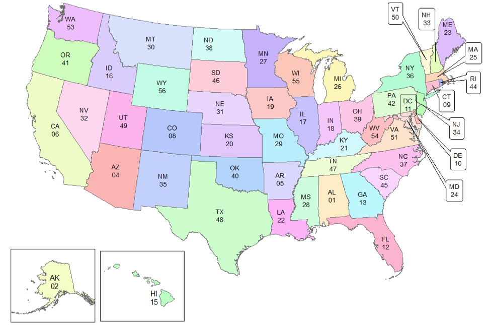
counties2 <- merge(counties, nhgis, by.x="GEOID", by.y="county2")And let’s limit our analysis to a few states in the Southeastern United States. That’s a practical decision - running maps for every county in the US takes a bit of time and computing power, but if we just do a few states these things can process faster. So let’s select Louisiana, Alabama, and Mississippi.
From Chen Zhang’s Blog
Let’s practice running spatial models using the percentage of residents that lack any form of health insurance as the dependent variable. Do you think the percentage of residents without any health insurance is randomly spread across different counties? Let’s start by looking at a plot for just that variable. We’ll use a yellow-to-green palette (YlGn).
tm_shape(counties3) + tm_polygons(style="quantile", col = "noinsurance", palette="YlGn") +
tm_legend(outside = TRUE, text.size = .8) 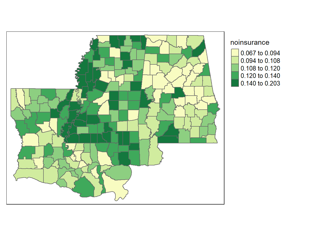
That looks pretty clustered. But we can figure out whether there are actual issues by running an OLS regression, and then observing the residuals. Let’s include the share of tourism employment, the percentage of residents over the age of 70, the poverty, and the income inequality as our independent variables. We’ll also include the state that each county is in, to account for the presence of different government programs that might impact residents throughout a state. We’ll save the regression output as ols.
##
## Call:
## lm(formula = noinsurance ~ tourismemp + over70pct + povpct +
##     gini + STATEFP, data = counties3)
##
## Residuals:
##       Min        1Q    Median        3Q       Max
## -0.051330 -0.013136 -0.001132  0.010752  0.056536
##
## Coefficients:
##              Estimate Std. Error t value Pr(>|t|)
## (Intercept)  0.105917   0.024267   4.365 2.01e-05 ***
## tourismemp   0.081673   0.043387   1.882  0.06119 .
## over70pct    0.206825   0.083325   2.482  0.01386 *
## povpct       0.219751   0.027283   8.054 6.33e-14 ***
## gini        -0.163687   0.054011  -3.031  0.00275 **
## STATEFP22    0.010093   0.003735   2.703  0.00746 **
## STATEFP28    0.021751   0.003488   6.235 2.51e-09 ***
## ---
## Signif. codes:  0 '***' 0.001 '**' 0.01 '*' 0.05 '.' 0.1 ' ' 1
##
## Residual standard error: 0.0199 on 206 degrees of freedom
## Multiple R-squared:  0.4422, Adjusted R-squared:  0.4259
## F-statistic: 27.21 on 6 and 206 DF,  p-value: < 2.2e-16
Remember that the dependent variable here is the % of residents without health insurance, so a positive coefficient indicates that variable is associated with people not having insurance. As such, the higher the share of employment in tourism, the larger the share of people over 70, and the higher the poverty rate the larger the uninsured population is in our data. As income inequality increases, the share of people without insurance decreases. The uninsured rate in Louisiana and Mississippi appear to be higher than Alabama when holding all else constant. Not that any of that is really our focus at the moment; you can interpret all of that the same as any other OLS. That’s actually true for all the models we’ll run in this section
First, let’s plot the residuals and see if they appear to be clustered. We’ll need to add our residuals as a new column to our dataset above first.
counties3$olsresiduals <- resid(ols)

tm_shape(counties3) + tm_polygons(style="quantile", col = "olsresiduals", palette="YlGn") +
tm_legend(outside = TRUE, text.size = .8) 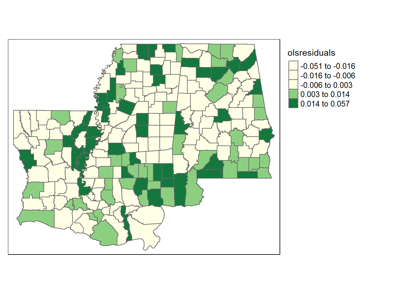
That definitely doesn’t look evenly distributed. But let’s check the Moran’s I and see if it tells us the residuals are geographically clustered. To run Moran’s I we’ll have to tell R which counties border other counties. That’s what the next 3 lines do, in a complicated way that I can’t even fully explain. We’re converting the original shapefile a few different ways, first to establish the network of neighbors and then restructuring it for the Moran’s I test. “rwm” is the name for the object that is a row-weights-matrix, because it is a matrix where the rows contain weights for which neighbors each county has. We’ll need the package spdep to use the command nb2listw, polyn2nb, and mat2listw.
library(spdep)
w <- poly2nb(counties3)
wm <- nb2mat(w, style='B')
rwm <- mat2listw(wm, style='W')
head(rwm$neighbours)
## [[1]]
## [1] 60 69 120 137 195
##
## [[2]]
## [1] 56 73 88 127 136 197 199
##
## [[3]]
## [1] 14 15 17 37 66 90 101 140
##
## [[4]]
## [1] 39 133 209
##
## [[5]]
## [1] 33 70 100 164
##
## [[6]]
## [1] 13 46 79 204Once we have that, we can use the final object “rwm” and our ols results “ols” with the Moran’s I test. The Moran’s I test for ols residuals is lm.morantest(), which sorta says what it is: a moran’s I test for lm (linear models). It is also in the package spdep.
##
##  Global Moran I for regression residuals
##
## data:
## model: lm(formula = noinsurance ~ tourismemp + over70pct + povpct
## + gini + STATEFP, data = counties3)
## weights: rwm
##
## Moran I statistic standard deviate = 2.9726, p-value = 0.002952
## alternative hypothesis: two.sided
## sample estimates:
## Observed Moran I      Expectation         Variance
##      0.102762940     -0.017172515      0.001627831
The p value indicates that the there is significant clustering for our residuals. As such, we’ll need to run spatial models to help correct for those problems. Let’s look at the code to correct for that, and then we can determine which model has best addressed that issue.
We’ll first run a spatial error model using the command errorsarlm(). That command is in the spatialreg package. I’m going to save the output from that regression for later as LMerr. There’s only one difference between the command below and running other regressions. We need to also insert a slightly differently structured object telling the command what counties are near other counties.
library(spatialreg)
LMerr <- errorsarlm(noinsurance ~ tourismemp + over70pct + povpct + gini+STATEFP, data = counties3, wm2)
summary(LMerr)
##
## Call:errorsarlm(formula = noinsurance ~ tourismemp + over70pct + povpct +
## gini + STATEFP, data = counties3, listw = wm2)
##
## Residuals:
## Min 1Q Median 3Q Max
## -0.054316 -0.013127 -0.001073 0.010121 0.055822
##
## Type: error
## Coefficients: (asymptotic standard errors)
## Estimate Std. Error z value Pr(>|z|)
## (Intercept) 0.0985144 0.0236764 4.1609 3.170e-05
## tourismemp 0.0783233 0.0434474 1.8027 0.071433
## over70pct 0.2228880 0.0834435 2.6711 0.007560
## povpct 0.2102767 0.0271859 7.7348 1.044e-14
## gini -0.1472172 0.0521931 -2.8206 0.004793
## STATEFP22 0.0105248 0.0045926 2.2917 0.021925
## STATEFP28 0.0218825 0.0041948 5.2166 1.822e-07
##
## Lambda: 0.2491, LR test value: 5.6239, p-value: 0.017718
## Asymptotic standard error: 0.099779
## z-value: 2.4965, p-value: 0.012543
## Wald statistic: 6.2324, p-value: 0.012543
##
## Log likelihood: 538.4768 for error model
## ML residual variance (sigma squared): 0.00036849, (sigma: 0.019196)
## Number of observations: 213
## Number of parameters estimated: 9
## AIC: -1059, (AIC for lm: -1055.3)And now let’s run the spatial lag model. That requires another command, lagsarlm(), also from the spatialreg package.
LMlag <- lagsarlm(noinsurance ~ tourismemp + over70pct + povpct + gini+STATEFP, data = counties3, wm2)
summary(LMlag)
##
## Call:lagsarlm(formula = noinsurance ~ tourismemp + over70pct + povpct +
## gini + STATEFP, data = counties3, listw = wm2)
##
## Residuals:
## Min 1Q Median 3Q Max
## -0.05272271 -0.01307079 -0.00052672 0.01082115 0.05313323
##
## Type: lag
## Coefficients: (asymptotic standard errors)
## Estimate Std. Error z value Pr(>|z|)
## (Intercept) 0.0839199 0.0242402 3.4620 0.0005362
## tourismemp 0.0769649 0.0417743 1.8424 0.0654174
## over70pct 0.1991472 0.0804857 2.4743 0.0133491
## povpct 0.2018760 0.0269189 7.4994 6.417e-14
## gini -0.1598154 0.0520014 -3.0733 0.0021171
## STATEFP22 0.0079015 0.0036977 2.1369 0.0326082
## STATEFP28 0.0163449 0.0039393 4.1492 3.337e-05
##
## Rho: 0.23968, LR test value: 6.7971, p-value: 0.0091307
## Asymptotic standard error: 0.088074
## z-value: 2.7214, p-value: 0.006501
## Wald statistic: 7.4059, p-value: 0.006501
##
## Log likelihood: 539.0634 for lag model
## ML residual variance (sigma squared): 0.00036681, (sigma: 0.019152)
## Number of observations: 213
## Number of parameters estimated: 9
## AIC: -1060.1, (AIC for lm: -1055.3)
## LM test for residual autocorrelation
## test value: 0.010984, p-value: 0.91653We’ll notice that for both models spatial autocorrelation is still a problem. You may also notice that it’s AIC is lower for the spatial lag than the spatial error model. Let’s run a Lagrange multiplier test to see which model is preferred though.
We can run the Lagrange multiplier test to determine which model is best. This is coming from the spdep package as well. It’s a long line of code, but ignore the summary command that wraps it (that’s just to get the output). We use the command lm.LMtests(), which we first give the name of our original model, “ols”, then the name of our queen’s neighbors weights, “wm2”, and then we give it a list of the models we want it to test, test=c(“LMlag”,“LMerr”). And then we get the output.
##  Lagrange multiplier diagnostics for spatial dependence
## data:
## model: lm(formula = noinsurance ~ tourismemp + over70pct + povpct
## + gini + STATEFP, data = counties3)
## weights: wm2
##
##       statistic parameter p.value
## LMlag    7.2451         1 0.00711 **
## LMerr    6.0123         1 0.01421 *
## ---
## Signif. codes:  0 '***' 0.001 '**' 0.01 '*' 0.05 '.' 0.1 ' ' 1
Here, the spatial lag model has the higher test statistic (7.2451 vs. 6.0123), so we would report that model and use it even though it has not completely corrected our problem. No model is perfect, it’s just about getting the one that is least imperfect. No where is that truer than using spatial data.